Bias Variance Tradeoff in Machine Learning

Bias, Variance, and Bias-Variance tradeoff are the most popular terms in machine learning and the most frequent questions asked in machine-learning interviews. To understand the concept of Supervised learning thoroughly, one must know these terms.

Whenever we talk about the machine learning model, one question quickly comes to mind: what is the accuracy of that model or, in similar terms, if that model predicts the output, what are the errors associated with that prediction, and how much?

Bias and Variance are those error-causing elements only. Knowledge about these errors will help diagnose the models and help reduce the chances of overfitting and underfitting problem. To proceed ahead, let’s quickly define these two terms,

Bias

To make the target function easier to learn, the simplifying assumptions made by the model are termed as bias. Suppose you have given, Input to a model as

X = [1,2,3,4,5,6], and corresponding output as, Y = [1,8,27,64,125,216].

Clearly, Y = X³ is the relation between input and output which is non-linear, and the model will try to learn. But what if our model can only learn linear functions? In that case, our model will try to fit a linear function between X and Y by minimizing the error. Here, the model assumed that X and Y form a straight line, and this assumption is biased.

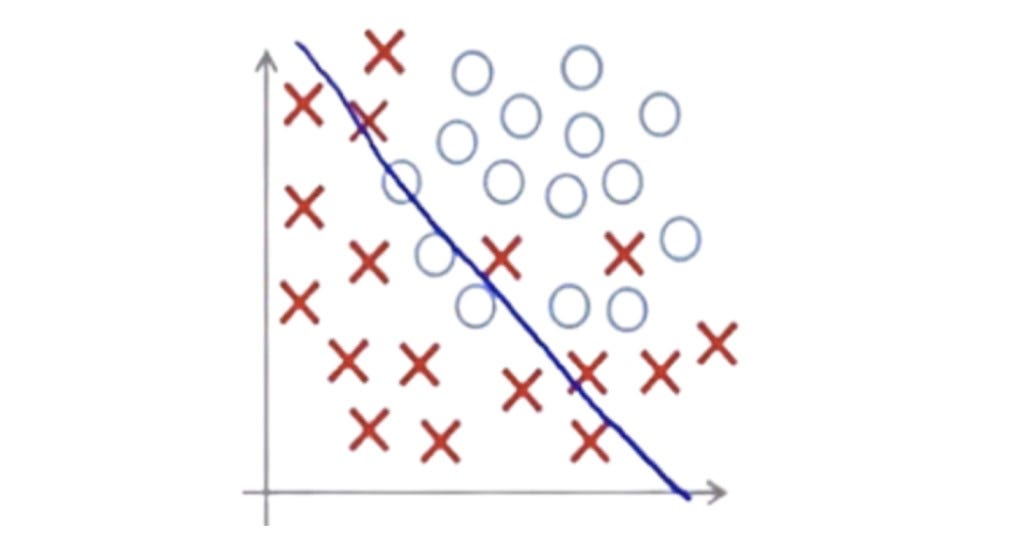
1. Low Bias:- Lesser assumption made about the target function

2. High Bias:- More assumptions made about the target function.

Error due to Bias:- The difference between the average expected prediction of our machine learning model and the actual value that we wanted to predict.

Variance

The estimated target function will change if different training data has been used for that model to train. And the amount by which that new estimated target function would change from the previously estimated target function is termed the variance.

For a better realization, let’s think, What model learns? We know that the model learns the weight matrices' entries and biases in data as an answer. If for the different datasets but similar use cases, these learned variables should not change too much.

Ideally, it should not change too much with the variation of the training data, which shows that our model can learn the underlying relations between input and output variables.

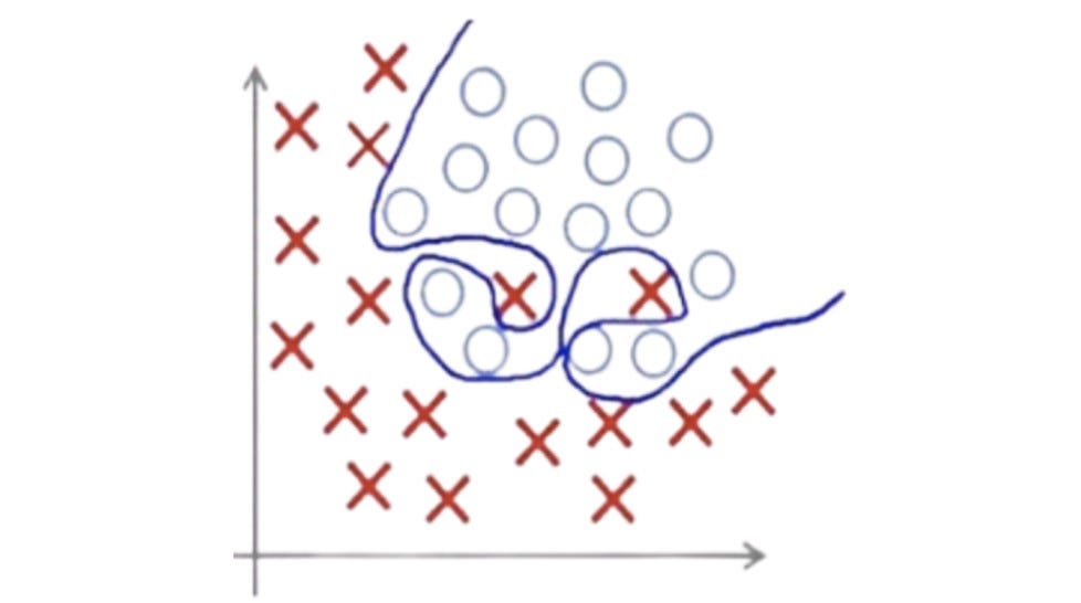
1. Low Variance:- Lesser variation in the model with the variation in training data. With a slight change in the input data, model prediction changes very little.
2. High Variance:- More variations in the model with the variation in training data. With a slight change in input data, model predictions vary significantly from the previous case.

Error due to Variance:- The error due to variance is the variability of a model prediction for a given data point. It also shows the spread of the data.

Graphical Illustration (BULL’S EYE DIAGRAM)

Suppose the inner-most circle (Red circle in diagram) is the target that the model wants to predict accurately. More the distance of prediction from Bull’s Eye, worse the prediction. Suppose the entire model building process can be repeated to get several separate hits on the bull’s eye target. Each dot in the below image represents each hit after retraining under the assumption that there will be some variations in the models after retraining. 

This entire process depends on data distribution also. Sometimes training data is from a good distribution, and predictions come close to the bull’s eye, and sometimes there may be many outliers present in the data, which can cause the scatter in the predictions.

We can represent the High/Low Bias/Variance scene from the below image.

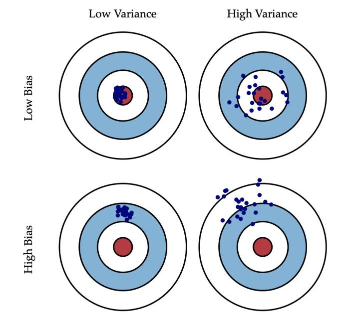
Credit: Scott Fortmann Roe

Mathematical Derivation

 (Requires Knowledge of Probability density function and expectation values)

Suppose Y is the target variable and X is the corresponding input variable. We may assume that there is one underlying relationship between these two variables like Y = f (X) + ε, where ε is the normally distributed error with mean = 0 and variance = σ², i.e., ε ~𝑁(0, σ²),

Now suppose our model is trying to fit this f, but it somehow fitted f^.

So the expected square error for any input variable X would be,

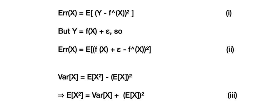
E(f) = f, as f is independent on dataset given E[ε] = 0, as noise mean is zero.

Hence,

And we already know, Var[ε] = σ²,

Now, from equation (ii), adding and subtracting E( f^(X)) inside the expectation function,

As we know, (a + b + c)² = a² + b² + c² + 2ab + 2bc + 2ca, hence,

Now, as f^(X) and ε are independent, f (X) is constant for a particular X value. So,

Now,

On a conclusion basis, we can say that

MSE = Bias² + Variance + Irreducible error

And for a better prediction, the error should be minimum.

That irreducible error is the noise term that can’t be reduced by any model. With a true model and infinite data to calibrate the model, we should be able to make the errors due to bias and variance close to 0 but still will not remove that irreducible error.

However, in a present world where we have imperfect models and finite data, there is a tradeoff between minimizing the bias and minimizing the variance.

But before proceeding ahead, let’s define two terms.

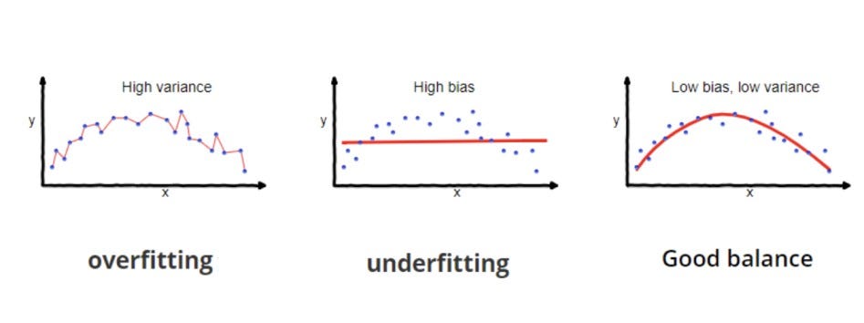
1. Underfitting:- A situation in which the model fails to capture the underlying pattern in the data. In this situation, the model usually suffers from high bias and low variance. This situation arrives when there is very little data to build an accurate model or when we try to fit a linear model on data having nonlinearities. These models are straightforward and hence fail in capturing complex relationships. E.g., Linear regression.
2. Overfitting:- A situation in supervised learning, in which the model starts capturing the noisy patterns along with the underlying patterns in data. In this situation, the model usually suffers from low bias and high variance. This situation arrives when we have a higher portion of noise in data. These are complex models and capable of learning complex functions. E.g., Decision Trees.

Bias-Variance Tradeoff

The goal of any supervised learning method is to achieve the condition of Low bias and low variance to improve prediction performance.

But the relationship between bias and variance is like:-

• If you increase the bias, a variance will decrease
• If you increase the variance, bias will decrease

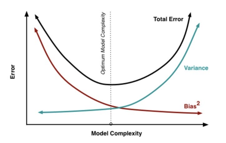
So overall, we try to achieve the optimum value at which our Total Error that can be minimized, which is Bias² + Variance, becomes minimum.

This is Bias — Variance Trade-Off.

Bonus Section

Now, We know about this tradeoff but, there are still some unanswered questions,

Q 1. How will we find that our model is suffering from High/Low Bias/Variance?

Q 2. What will we need to do to reduce such errors?

To answer these questions, let’s visualize one scenario,

Suppose we are building a model to solve a supervised learning problem. We have two kinds of errors,

1. Training Error:- Machine Learning model performance on data which is used for its training.
2. Testing Error:- Machine Learning model performance on data which is unseen to model.

• If the gap between Zero Error and Training error is very high, the model suffers from High Bias. To reduce this error, one can try increasing the complexity of the model (Try to fit a more complex model).
• If the gap between zero and testing errors is shallow, but the gap between training and testing errors is very high, the model suffers from High Variance. To reduce this gap, one can try these steps sequentially,
  1. Filter the data first and then train
  2. Increase the amount of training data.
  3. Dropout some percent of learnings (Using Regularizers).
  4. Decrease model complexity.

Possible Interview Questions

Conclusion

In this article, we explained one of the most important topics in machine learning that affects the choice of different models. We first defined the terms of Bias and Variance and later explained how they produce underfitting and overfitting problems in machine learning. We also explained the concept of bias-variance tradeoff using graphical representation as well as the mathematical perspective. In the bonus section, we explained how we could decide whether our model is suffering from an underfitting or overfitting problem and the cure for that. We hope you enjoyed the article.

References

1. Andrew Ng Courses
2. http://scott.fortmann-roe.com/docs/BiasVariance.html

Enjoy Learning! Enjoy Mathematics! Enjoy Algorithms!