Guide to Implement Machine Learning Model using Python

In today's era of machine learning, the support of libraries and frameworks is easily accessible. We can build the entire machine learning pipeline ranging from dummy data availability to model development & deployment with just a few lines of code. However, these supports are handy and help us treat algorithms as black boxes. It is good from the perspective of an application. But from the learning perspective, It would be highly recommended to know the working methodologies for algorithms that we are using to build any solution.

In this article, we will implement a basic machine learning project without using frameworks like Scikit-learn, Keras, or Pytorch. We will use the NumPy library for numerical operations and Matplotlib to visualize the graphs to build an ML model from scratch. So let's first define a simple dummy problem statement and sequentially build the solution using Machine Learning.

Problem Definition

Let's take a simple problem to be able to follow each step thoroughly. As we know, machines learn a mapping function from input to output variables. Similar to that, here we want our machine to learn a mapping function following this equation:

problem definition function for coding from scratch blog

If we notice, it's a quadratic equation, and Y is continuous; hence it is a Regression problem that requires data in the supervised format. Supervised data format means we will know the target/output variables for some sample of input available. Let's create the dummy data for our problem statement.

Data Generation

We can choose some random values of X for this problem and generate the corresponding Ys using the above formulae coded in python. We will use Numpy's arange function to pick values from the range of -5 to +5 after every 0.2 unit interval. For example, [-5, -4.8, -4.6, …, +4.6, +4.8]. Note: +5 is excluded; hence we will have 50 data samples (Think how!).

X = np.arange(-5,5,0.2)
#generating the corresponding Y
Y = -1*(X**2 + X - 2)
# checking the length of Y
print("Total Samples = ", len(Y))

We have the dataset now and can proceed ahead with the further steps. Data is considered the heart of ML, and the more we know about it, the better we will be able to depict the behavior of our algorithms. So let's first visualize it and do some pre-processing on it.

Data Analysis and Pre-processing

Let's first visualize the data that we generated in the previous step. For plotting the curve, we will use the Matplotlib library.

from matplotlib import pyplot as plt

plt.figure("Data Figure")

plt.scatter(X, Y, color='red', label='data')

plt.xlabel('X', fontsize=16)
plt.ylabel('Y', fontsize=16)

plt.grid()
plt.show()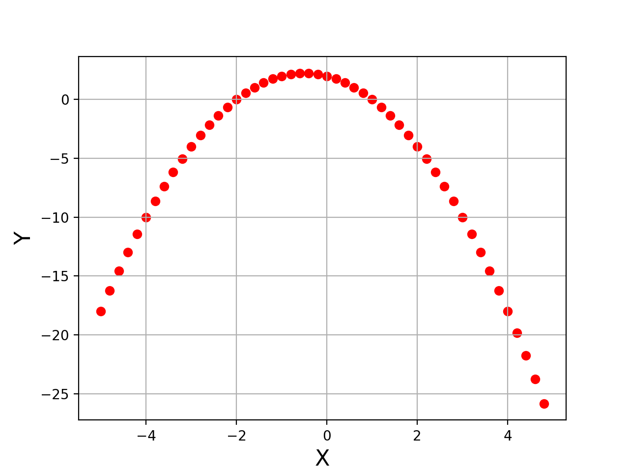

Data generated without noise in coding ml from scratch

Noise Addition

Learning this straightforward function would be much easier for machines. To make it slightly challenging, let's add some impurity in the data,

Data with gaussian noise of mean 0 and variance sigma_square for coding ML from scratch blog

Where f is the given function to learn (-X² -X +2), and ε is the impurity (or noise) having zero mean and σ² variance. To add this impurity in the data, we will use the random.normal function present in the Numpy library, which takes three input parameters as mean, variance, and total samples to be generated. We can control the magnitude of this noise by changing the value of magnitude in the code below.

magnitude = 2
Y = -1*(X**2 + X - 2) + magnitude*np.random.normal(0,1,len(X))

After this, data will look something like shown in the figure below.

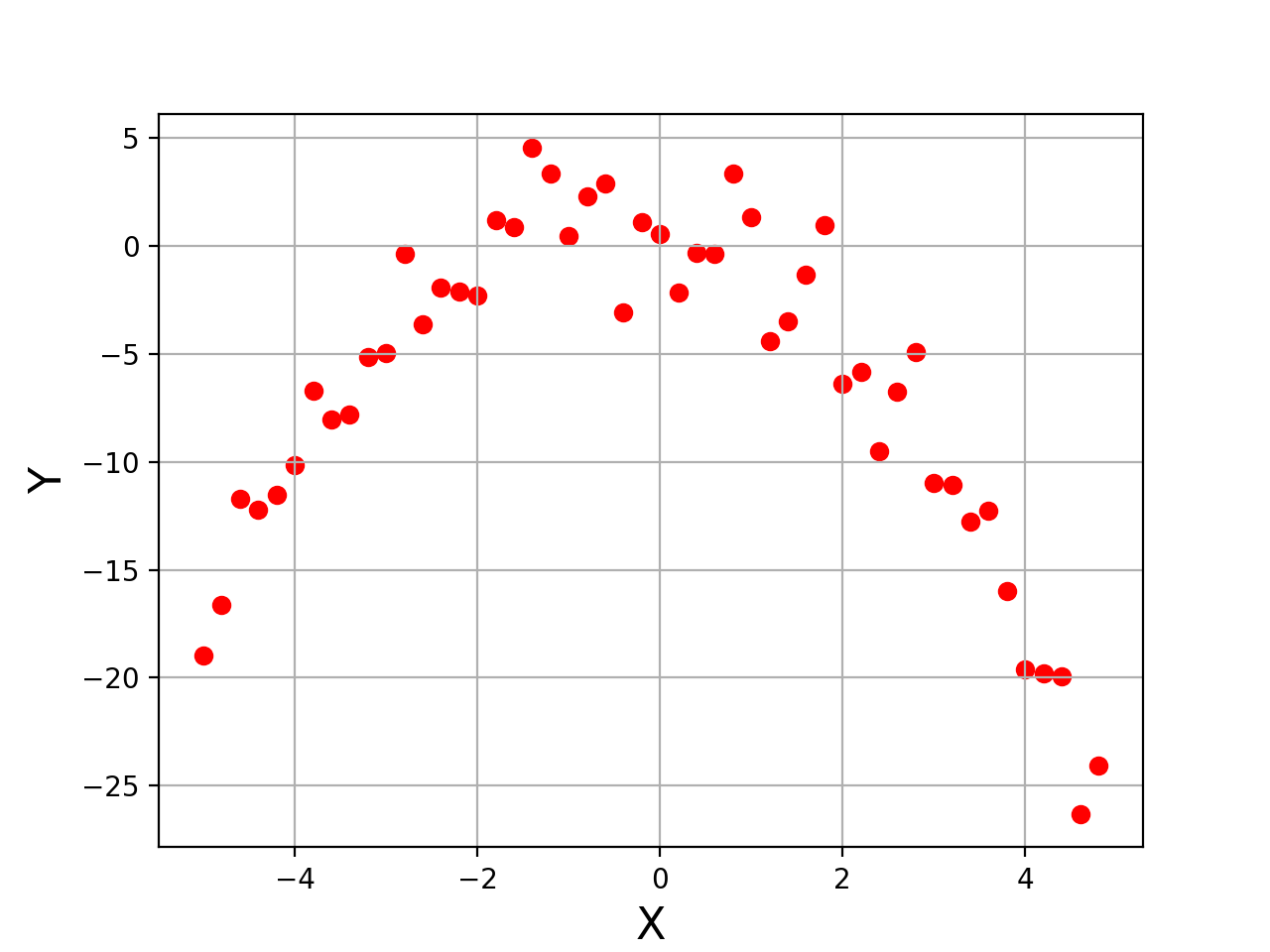
Data visualization with noise addition

Please note that we have added noise directly in the target variable. Let's use this data as our final dataset on which we want to fit a 2-degree polynomial.

Parametric formulae of the quadratic equation

If somehow using ML, we would be able to find that θ0≈2, θ1≈-1, θ2≈-1, our job will be done. We know that machines learn weight and bias matrices to learn the mapping function. If we represent the above equation using the weight and bias matrix multiplication, it will look like this:

Matrix based representation of parametric equation

Feature Formation

If we represent the dataset in the tabular format, one column would be X that we picked randomly in [-5, 5], and the second column would be the calculated Y from the data generation step. We would need to make another column of X² as a new feature to make it compatible with the above equation. The function below make_polynomial_features will do that for us. It will take the input of X and Y, will calculate the X², and concatenate it with the existing X value.

def make_polynomial_features(X, Y):

	X1 = np.reshape(X, (X.shape[0], 1))
	X2 = X**2
	X2 = np.reshape(X2, (X2.shape[0], 1))
	new_data = np.concatenate((X1, X2), axis=1)

	Y1 = np.reshape(Y, (Y.shape[0], 1))
	new_data = np.concatenate((new_data, Y1), axis=1)

	return new_data

X1 = make_polynomial_features(X, Y)
X = X1
np.random.shuffle(X)

Shuffle the data

If we feed the input in an increasing order starting from -5 to +5, the model will probably get a sense that input contains some increasing pattern. To avoid that, we need to shuffle the data samples. If we notice in the above code, we stacked the target variable into the final complete data to ensure that the corresponding Y position should remain the same if we shuffle the input data X.

Mathematical Understanding

Now, we have the data ready for our Machine Learning algorithm. We will be using the famous gradient descent algorithm to help find accurate values of θs. Our data is free from outliers as we have generated it from a fixed polynomial equation and added slight noise. So, we can use MSE (mean squared error) as our cost function.

We can also represent the relationship between X and Y as,

Relationship between Y and X in terms of weight and bias

We know that the updates in the gradient descent happen in a specific way shown in the equation below, where J represents the cost function (MSE in our case).

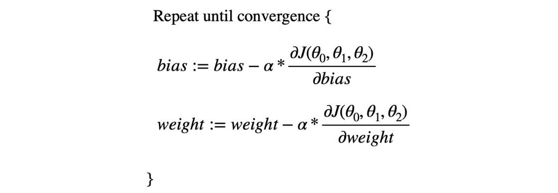
Gradient descent pseudo code enjoyalgorithms

And in the case of MSE J(θ0, θ1, θ2) = error², we know the gradients are like,

Gradient calculation equations 1

Gradient calculation equations 2

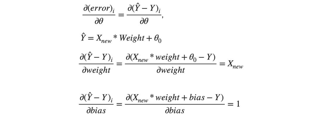
θ0 is the bias and the [θ1, θ2].T is the Weight matrix for our use case. Hence the terms in the gradient descent will look like this,

Updates of weight and bias values

Matrix Dimension Verification

We are playing with the matrices, so we should cross-check the dimensional validity.

Dimensions of different matrices

In the update of weight term, we need to multiply error and X_new, such that it produces (2 X 1) matrix then only addition or subtraction with weight matrix will be possible. For that, we will use the dot product between error and Xnew matrices. If we operate Transpose(Xnew)*error, then a (2 X 50) matrix will get multiplied to a (50 X 1), resulting in a (2 X 1) matrix. This proves that the equations we derived follow the expectations.

Model Building

Too much maths!! But, now we know everything that we need. So, let's code our gradient descent algorithm from scratch.

Prediction Function

def prediction(weight, bias, X):

	Y_predicted = np.dot(X, weight) + bias

	return Y_predicted

The above function prediction gives us the predicted value for a given weight, bias, and input matrices. This function will be required to calculate expected values after every update done in the gradient descent implementation. The learning rate is fixed for gradient descent, so let's keep a small value of 0.001, and we want the parameters to get updated 1000 times, assuming that those many steps will be sufficient to find the minima of the cost function J.

def fit_ml(X_train, Y_train, learning_rate=0.001, iterations=1000):

	num_samples, num_features = X_train.shape

	print("number of samples = ",num_samples)
    print("number of features = ",num_features)
    
	weight = np.zeros(num_features)
	bias = 0.1

	for i in range(iterations):

		Y_predicted = prediction(weight, bias, X_train)

		dw = (1/num_samples)*2*np.dot(X_train.T, (Y_predicted - Y_train))
		db = (1/num_samples)*2*np.sum((Y_predicted - Y_train))

		weight = weight - learning_rate*dw
		bias = bias - learning_rate*db

	return weight, bias

The function fit_ml is ready to be used.

Data Splitting

We can not use 100% data for training purposes. To check the model's performance, we also need to test it on some unseen data. That's why we will split the available dataset into training and testing samples. As the samples are shuffled, we can choose the first 80% data samples for training and the rest 20% for testing the model performance.

def make_spliting(data, split_percentage=0.8):

	X_train = X[:int(split_percentage*(len(X))),:-1]
	Y_train = X[:int(split_percentage*(len(X))),-1]

	print(X_train.shape, Y_train.shape)

	X_test = X[int(split_percentage*(len(X))):, :-1]
	Y_test = X[int(split_percentage*(len(X))):,-1]

	return X_train, Y_train, X_test, Y_test

X_train, Y_train, X_test, Y_test = make_spliting(X)

plt.figure("Data")
plt.scatter(X_train[:,0], Y_train, color='red', label='train_data')
plt.scatter(X_test[:,0],Y_test,color='green',label='test_data')
plt.xlabel("Samples", fontsize=16 )
plt.ylabel("Y", fontsize=16 )
plt.legend(loc="upper right")
plt.grid()
plt.show()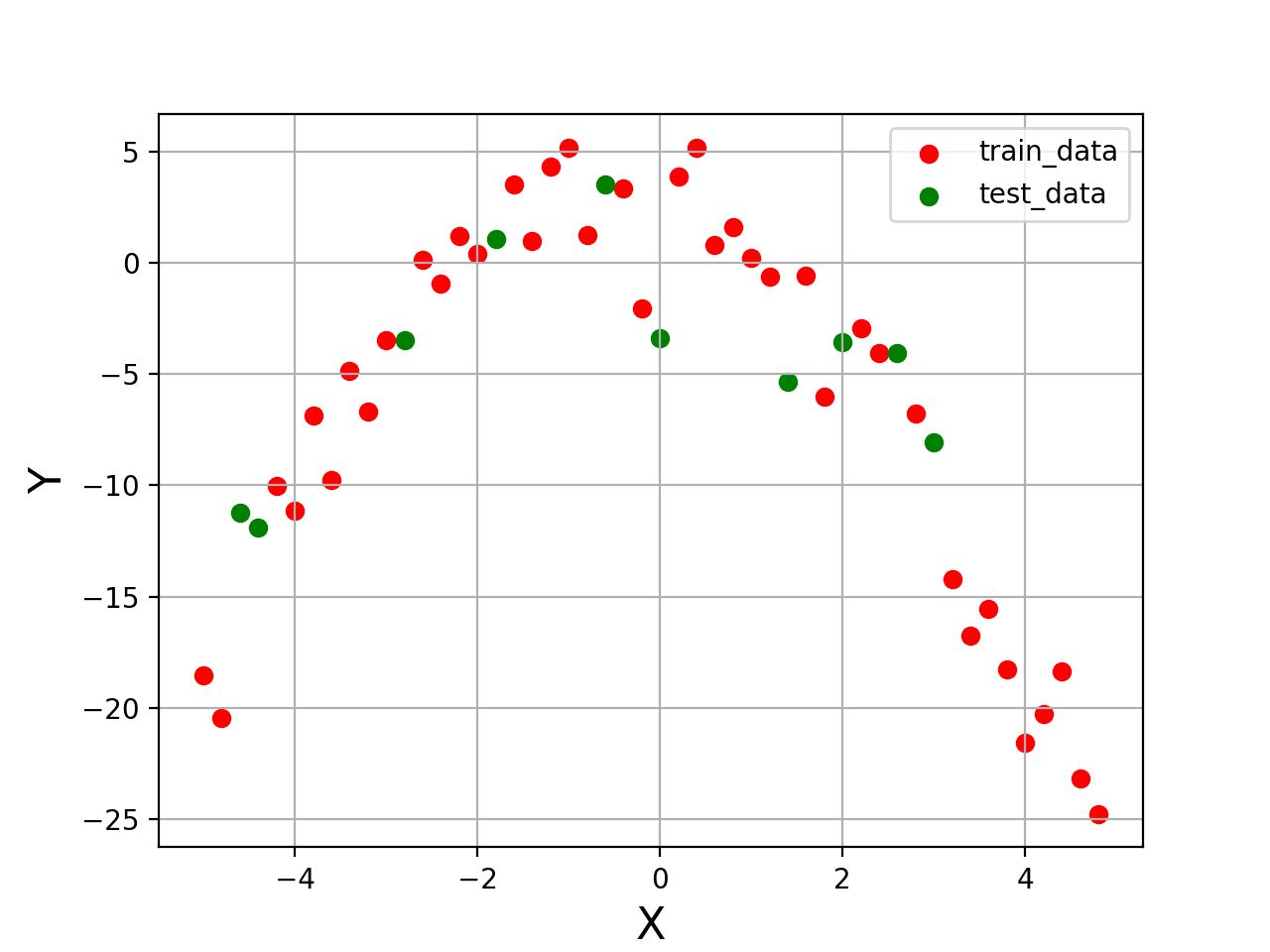

Training and testing data visualization for coding ml from scratch

Evaluation Metric

It's a regression problem, and hence MSE can be used to evaluate the performance.

def evaluation_mse(Y_predicted, Y_actual):

	m = len(Y_actual)
	mse = 0
	
    for i in range(m):

		mse = mse + (Y_predicted[i] - Y_actual[i])**2

	MSE = (1/m)*mse
    return MSE

Training

We are ready to train our Machine Learning algorithm. After calling the fit_ml function, we will have the learned parametric values, and we will say that our machine has learned.

#Below line will give us the weight and bias matrix values
weight, bias = fit_ml(X_train, Y_train)

print("Training Done")

#Below line is used to predict on train data
Y_train_pred = prediction(weight, bias,X_train)

print("Mean Squared Error = ",evaluation_mse(Y_train_pred, Y_train))

plt.figure("Training")
plt.scatter(X_train[:,0], Y_train, color='red', label='train_data')
plt.scatter(X_train[:,0], Y_train_pred, label='prediction')
plt.xlabel("X", fontsize=16 )
plt.ylabel("Y", fontsize=16 )
plt.legend(loc="upper right")
plt.grid()
plt.show()



###Mean Squared Error =  5.584458137818953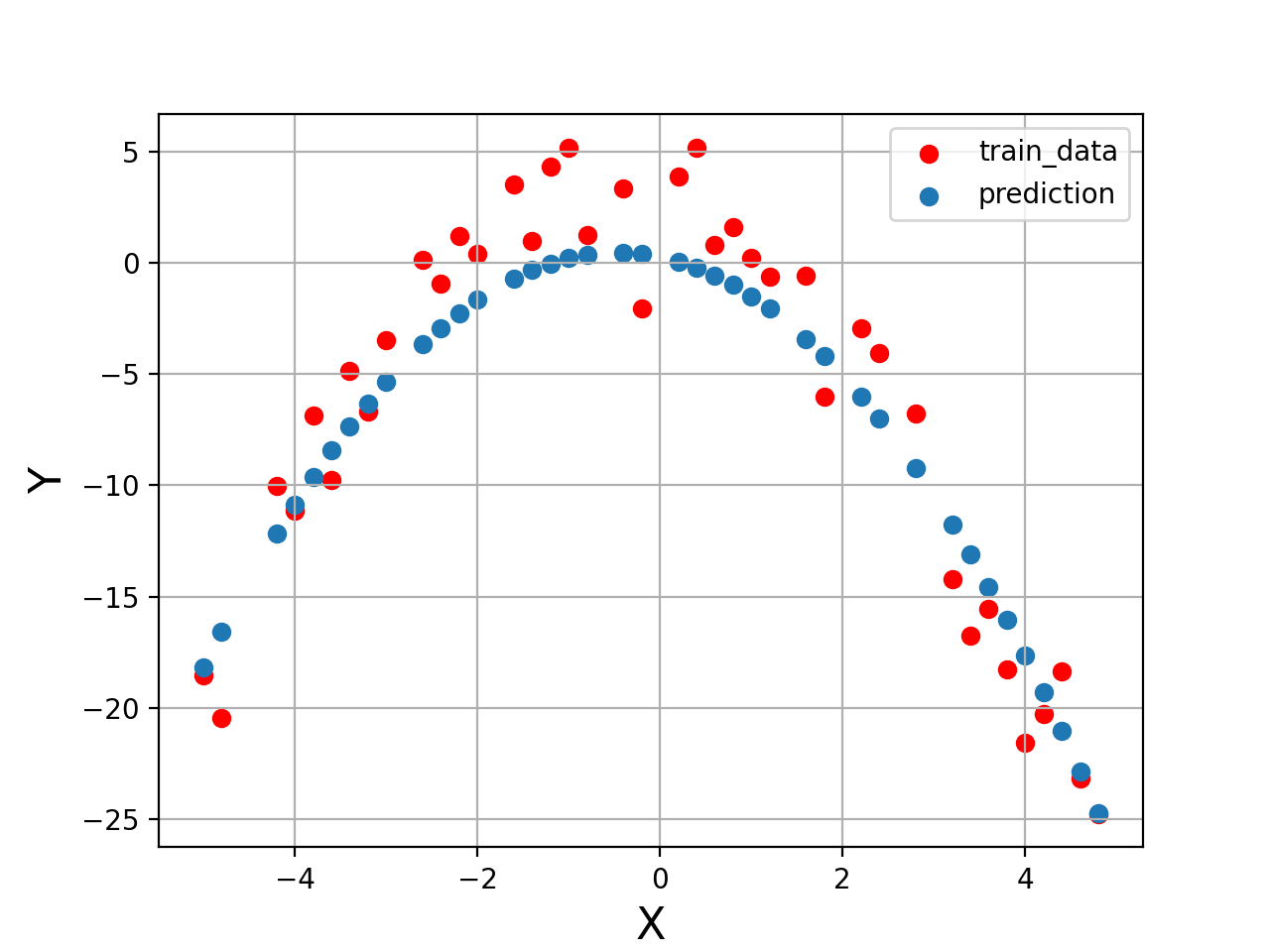

Model results on training data for coding ml from scratch

Testing

Now, we have the trained parameters (Weight and Bias matrices). We can test the accuracy of these values on utterly unseen data samples. So, let's do that.

Y_test_pred = prediction(weight, bias, X_test)

print("Mean Squared Error = ",evaluation_mse(Y_test_pred, Y_test))

plt.figure("Testing")
plt.scatter(X_test[:,0], Y_test, color='green', label='test_data')
plt.scatter(X_test[:,0], Y_test_pred,label='prediction')
plt.xlabel("X", fontsize=16 )
plt.ylabel("Y", fontsize=16 )
plt.legend(loc="upper right")
plt.grid()
plt.show()



#Mean Squared Error = 5.86669209809574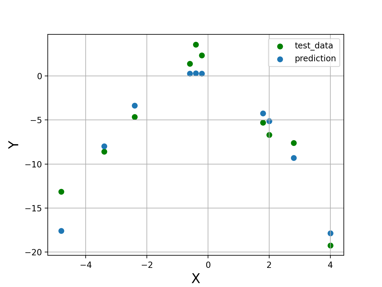

Model results on testing data for coding ML from scratch

Testing on all available data and Drawing a solid line

We can not draw a solid line directly because samples are shuffled, and if we use the plot function of matplotlib, it will be a mess. To sort this mess, we need to sort samples according to X values and then use their corresponding Y values to plot the solid line.

Y_pred = np.reshape(prediction(weight, bias, X1[:,:-1]), (len(X1[:,:-1]), 1))

plot_x = np.concatenate((np.reshape(X1[:,0], (len(X1[:,0]),1)),Y_pred), axis=1)

plot_x1 = np.concatenate((np.reshape(X1[:,0], (len(X1[:,0]),1)),np.reshape(Y, (len(Y),1))), axis=1)
plot_x = plot_x[plot_x[:, 0].argsort(kind='mergesort')]


plt.figure("All plot")
plt.scatter(plot_x[:,0],Y, color='red', label='Actual Values')
plt.plot(plot_x[:,0],plot_x[:,1], label='predicted function')
plt.xlabel("X", fontsize=16)
plt.ylabel("Y", fontsize=16)
plt.legend(loc="upper right")
plt.show()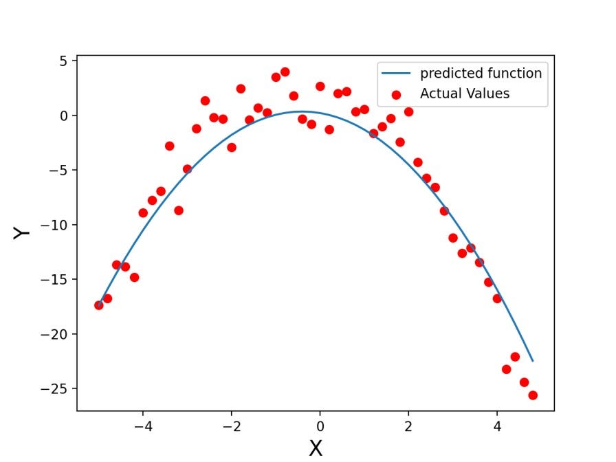

Model results on all data with solid line for coding ml from scratch

Keeping everything in one place

The complete code can be seen below.

import numpy as np

def prediction(weight, bias, X):

	Y_predicted = np.dot(X, weight) + bias

	return Y_predicted


def fit_ml(X_train, Y_train, learning_rate=0.001, iterations=1000):

	#initialize the weights

	num_samples, num_features = X_train.shape

	print(num_samples, num_features)

	weight = np.zeros(num_features)
	bias = 0.1


	for i in range(iterations):

		#print("Iteration no.: ", i)

		Y_predicted = prediction(weight, bias, X_train)

		dw = (1/num_samples)*2*np.dot(X_train.T, (Y_predicted - Y_train))
		db = (1/num_samples)*2*np.sum((Y_predicted - Y_train))

		weight = weight - learning_rate*dw
		bias = bias - learning_rate*db

	return weight, bias



def evaluation_mse(Y_predicted, Y_actual):

	m = len(Y_actual)
	mse = 0
	for i in range(m):

		mse = mse + (Y_predicted[i] - Y_actual[i])**2

	MSE = (1/m)*mse
	return MSE

X = np.arange(-5,5,0.2)

Y = -1*(X**2 + X - 2) + 2*np.random.normal(0,1,len(X))

from matplotlib import pyplot as plt
plt.figure("Data Figure")

plt.scatter(X, Y, color='red', label='data')
plt.xlabel('X', fontsize=16)
plt.ylabel('Y', fontsize=16)

plt.grid()
plt.show()


def make_polynomial_features(X, Y):

	X1 = np.reshape(X, (X.shape[0], 1))

	X2 = X**2
    X2 = np.reshape(X2, (X2.shape[0], 1))
    new_data = np.concatenate((X1, X2), axis=1)

	Y1 = np.reshape(Y, (Y.shape[0], 1))
    new_data = np.concatenate((new_data, Y1), axis=1)

	return new_data

#print(len(X))

X1 = make_polynomial_features(X, Y)
X = X1
np.random.shuffle(X)

def make_spliting(data, split_percentage=0.8):

	X_train = X[:int(split_percentage*(len(X))),:-1]
	Y_train = X[:int(split_percentage*(len(X))),-1]

	print(X_train.shape, Y_train.shape)

	X_test = X[int(split_percentage*(len(X))):, :-1]
	Y_test = X[int(split_percentage*(len(X))):,-1]

	return X_train, Y_train, X_test, Y_test

X_train, Y_train, X_test, Y_test = make_spliting(X)

plt.figure("Data")
plt.scatter(X_train[:,0], Y_train, color='red', label='train_data')
plt.scatter(X_test[:,0],Y_test,color='green',label='test_data')
plt.xlabel("X", fontsize=16 )
plt.ylabel("Y", fontsize=16 )
plt.legend(loc="upper right")
plt.grid()
plt.show()

weight, bias = fit_ml(X_train, Y_train)

print("Training Done")

Y_train_pred = prediction(weight, bias,X_train)
print("Mean Squared Error = ",evaluation_mse(Y_train_pred, Y_train))

Y_test_pred = prediction(weight, bias, X_test)
print("Mean Squared Error = ",evaluation_mse(Y_test_pred, Y_test))

Y_pred = np.reshape(prediction(weight, bias, X1[:,:-1]), (len(X1[:,:-1]), 1))
plot_x = np.concatenate((np.reshape(X1[:,0], (len(X1[:,0]),1)),Y_pred), axis=1)
plot_x1 = np.concatenate((np.reshape(X1[:,0], (len(X1[:,0]),1)),np.reshape(Y, (len(Y),1))), axis=1)

plot_x = plot_x[plot_x[:, 0].argsort(kind='mergesort')]


plt.figure("All plot")
plt.scatter(plot_x[:,0],Y, color='red', label='Actual Values')
plt.plot(plot_x[:,0],plot_x[:,1], label='predicted function')
plt.xlabel("X", fontsize=16)
plt.ylabel("Y", fontsize=16)
plt.legend(loc="upper right")
plt.show()

plt.figure("Training")
plt.scatter(X_train[:,0], Y_train, color='red', label='train_data')
plt.scatter(X_train[:,0], Y_train_pred, label='prediction')
plt.xlabel("X", fontsize=16 )
plt.ylabel("Y", fontsize=16 )
plt.legend(loc="upper right")
plt.grid()
plt.show()


plt.figure("Testing")
plt.scatter(X_test[:,0], Y_test, color='green', label='test_data')
plt.scatter(X_test[:,0], Y_test_pred,label='prediction')
plt.xlabel("X", fontsize=16 )
plt.ylabel("Y", fontsize=16 )
plt.legend(loc="upper right")
plt.grid()
plt.show()

Indeed an extended code. But you know, this same thing can be done within 10–15 lines using advanced machine learning frameworks. Not only this, but the codes used in the frameworks will be highly efficient as they will be using multithreading processes. That's how their code takes significantly lesser time and space compared to ours.

Conclusion

In this article, we successfully built a Machine Learning model by coding from scratch. Through this article, we demonstrated how exactly a machine learning algorithm works using the gradient descent algorithm. We hope you enjoyed the article.

Enjoy Learning! Enjoy Coding! Enjoy Algorithms!

Implement Machine Learning Model using Python from Scratch