Cost Function and Learning Process in Machine Learning

Humans learn through various methods such as practice, study, experiences, discussions, etc. On the other side, modern computers use machine learning techniques to learn similarly to simulate human intelligence. So obvious curiosity for us to know how exactly a machine learns something when it is non-living. In this blog, we'll dive into the mechanism through which a machine tries to mimic the learning process of humans. We will also discuss the concept of cost functions and the complete learning process of computers via machine learning.

Key takeaways from this blog

After reading this blog, we will gain an understanding of the following:

• How to evaluate the intelligence of a machine?
• The basic concept behind the cost function.
• The steps involved in the learning process for machine learning algorithms.
• How a machine stores its learned information.

Now, let's start with the first fundamental question.

How do we check intelligence of a machine?

In machine learning, we expect machines to mimic human intelligence by learning from historical data. In other words, machines learn the mapping function from input data to output data based on the past data provided.

The critical question is: How do we assess the learning progress of machines? Most of us may think: Isn't it when machines stop making errors or mistakes? Yes! Precisely the same way. But this learning process is divided into multiple steps. To understand this process thoroughly, let's take one data set and visualize learning steps in detail.

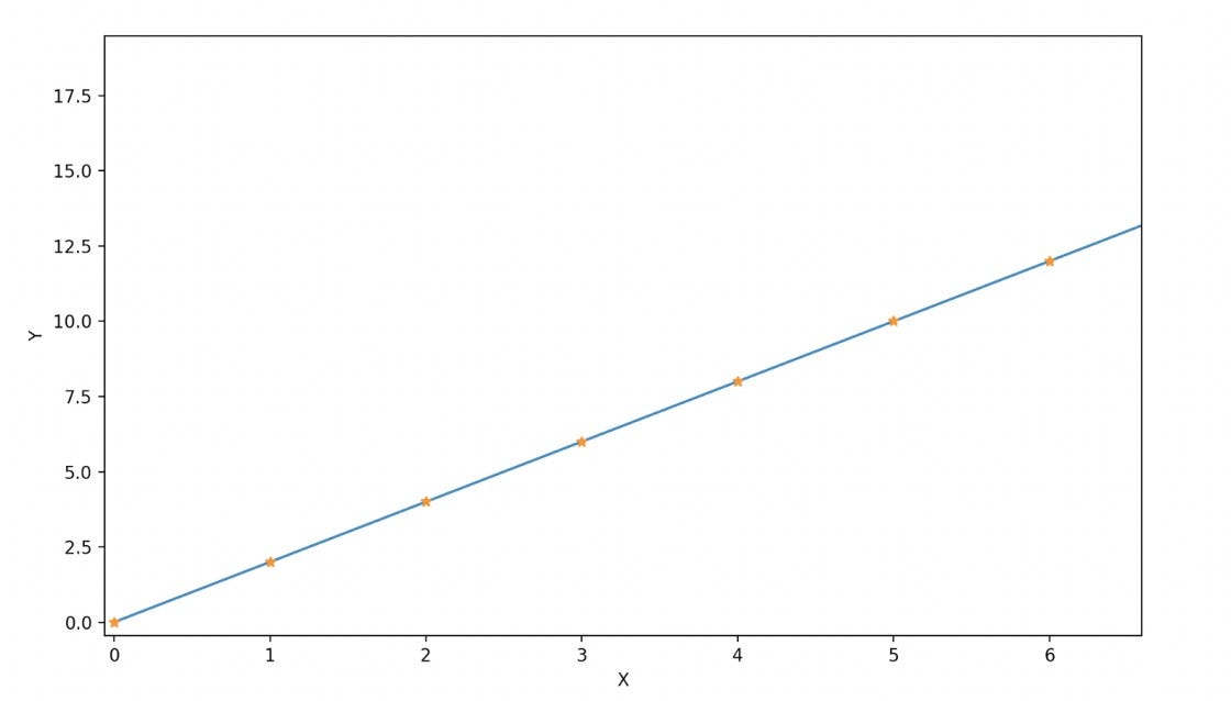
Suppose we have a historical dataset that consists of input and output pairs from a straight-line function, f(X) = 2X. We want our machine to learn this function automatically by analyzing the provided data, where X represents the input and f(X) = Y represents the output.

(X,Y) = [(0,0), (1,2), (2,4), (3,6), (4, 8), ..., (50, 100)]
X = [0, 1, 2, ..., 50]
Y = [0, 2, 4, ..., 100]

#There are 51 samples.

If we represent these (X, Y) points in the cartesian 2D plane, then the curve will be similar to what is shown in the image below.

Now, suppose we need the machine to learn a "linear" function of the form:

Our task is complete if the machine determines the suitable value for θ1, such that the equation holds for historical data pairs (input and output). For the given data samples, the "ideal" value of θ1 is 2. But the question is, how will machines find this value? Let's explore.

Steps involved in the learning process of machine learning algorithms

Step 1: Unintentionally make the mistake

The machine will randomly select a value for θ1. Let's say it chooses θ1 = 1, then estimates the output, Y' = 1 * X, which is different from the actual output Y. Now, we have two outputs: Y(actual output) and Y' (predicted output).

X = [0, 1, 2, ..., 50]
Y'= [0, 1, 2, ..., 50]

Step 2: Realization of the mistake

To determine how incorrect its initial guess of θ1 was, the machine will calculate the difference between the estimated outputs (Y') and the actual outputs (Y). This difference, or error, will be used to gauge the initial accuracy of the guess.

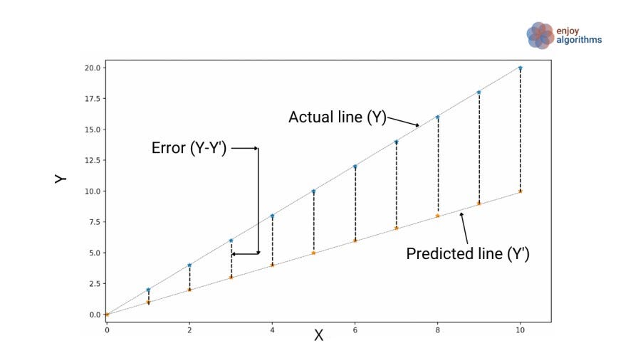
We have 51 data samples, so to take account of all the samples, we define an average error over all the data samples.

It's important to understand that our goal is to minimize this error as much as possible. In other words, our objective is to minimize the average error, and this average error is known as the cost function in machine learning. We will learn details about a cost function in our later blog on Loss and Cost Functions in Machine Learning.

Step 3: Rectifying the mistake

Now the machine will keep adjusting the value of θ1 to reduce the average error. If we plot the average error (or cost function) against various values of θ1 that it selects randomly, we will obtain a curve, as shown in the image below.

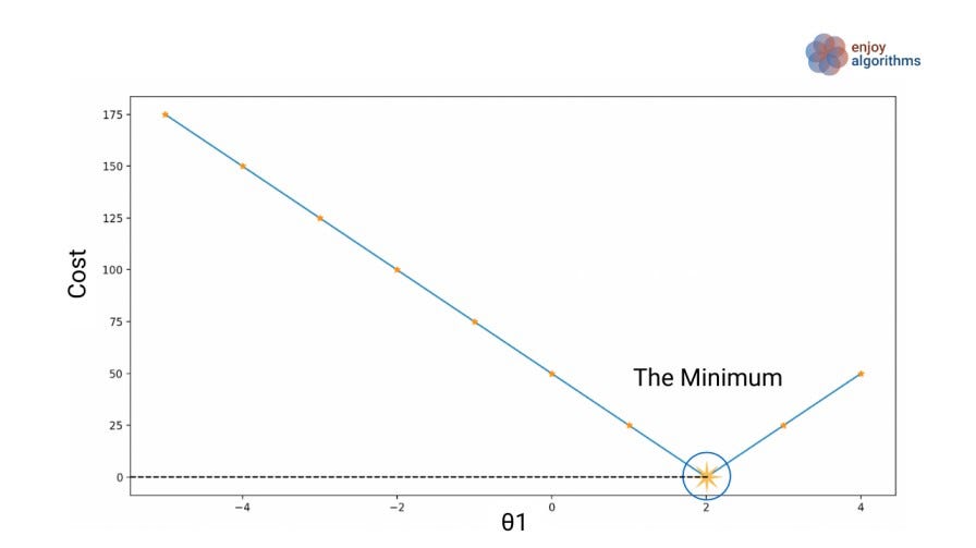
Here our objective is to minimize the cost function, and from the above graph, we can sense that for θ1 = 2, the value of the cost function would be minimal. The critical question is: How machine will adjust the value of θ1? For this, it will use optimization algorithms like gradient descent. In the gradient descent algorithm, the machine calculates the gradient of the cost function with respect to θ1, which represents the rate of change of the cost function.

• If the gradient is positive, the machine decreases the value of θ1.
• If the gradient is negative, the machine increases the value of θ1.
• This process continues until the cost function reaches its minimum value. At this point, the machine has found the optimal value of θ1.

Step 4: Learning from mistakes

The optimization process described above enables the machine to continually adjust the value of θ1 and reduce the average error (ultimately finding the best-fit line for the data). When it determines that θ1 = 2 results in the minimum of the cost function, it will store this value in memory and at this point, we can say that the machine has learned.

Step 5: Applying this learning

Now, if we provide the machine with a new value of X that it hasn't seen before, such as X = 500, it will simply use input X and apply it to the equation θ1*X, i.e. 2*500 = 1000.

It's important to note that this problem is relatively simple, as we only need to learn one parameter and estimate it by minimizing the cost function. However, things become more complex when we have multiple parameters to learn. Let's explore that scenario in the following steps.

Learning two parameters at the same time

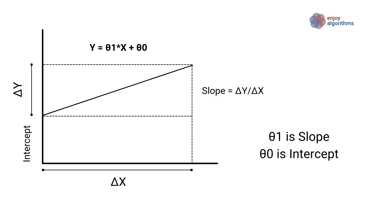
The general straight-line equation seems to be in the form of:

Where θ1 corresponds to the slope and θ0 is the intercept.

Suppose we want to estimate a linear function from our historical data from a linear equation Y = X + 1 (θ1 = 1 and θ0 = 1). Note: We selected a basic example so learners can follow the process quickly.

X = [0,1,2, ...., 50]
Y = [1,2,3, ...., 51]

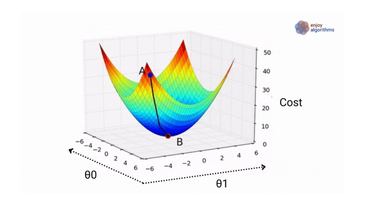
Compared to the previous scenario, we now need to determine the values of θ1 and θ0. Let's assume that the cost function is similar to what we saw before. To better understand the relationship, take a look at the figure below. It shows three dimensions, representing how parameters θ1 and θ0 impact the cost function.

Let’s again go step-wise through the complete process.

Step 1: Unintentionally make the mistake

Now the machine will randomly choose values for θ0 and θ1 (let's say it selects θ0 = 6 and θ1 = -6). Using these values, it will calculate Y', which is Y' = -6X + 6. This will be the location of point A in the above image.

Step 2: Realization of the mistake

The machine has both actual value (Y) and estimated value (Y') based on its initial random guess for parameters. To evaluate the accuracy of its prediction, the machine will calculate the average error or cost function for all input samples. This process is similar to what was described in the previous example.

Step 3: Rectifying the mistake

Now the machine will use an optimization algorithm like gradient descent to adjust parameters θ0 and θ1 so that the cost function will be minimum. In other words, the machine is trying to reach point B in the image.

Suppose, after trying several combinations of θ0 and θ1, the machine found that θ0 = 0.9999 and θ1 = 1.0001 produced the minimum cost function. Unfortunately, it missed checking the cost function at θ0 = 1 and θ1 = 1. Why do such situations occur in the optimization of a cost function? Here are some possible reasons:

• The algorithm may only be able to check a limited number of combinations of parameters, or it may have limited precision in its calculations. As a result, the machine may miss a combination of parameters that would have produced a lower cost function value.
• Another reason could be (Not applied to the above scenario because there is only one minimum): Optimization algorithm may be stopping at a local minimum rather than a global minimum, which is the actual minimum value of the cost function across all possible combinations of parameters.

We will learn the detailed working of the gradient descent algorithm in our next blog.

Step 4: Learning from mistakes

Now the machine will store two parameters as "learning" (θ0 = 0.9999 and θ1 = 1.0001) learned after trying various combinations of these parameters. We know these parameters are not perfectly correct, but our machine could only find these values within the given time limit.

Similarly, as the number of parameters increases, machines must find suitable values for all of them in a multi-dimensional space. Now the learning is complete, let's discuss how machines store these learnings as humans do in their memories.

How does a machine store its learnings?

Machines use matrices to store the perfect values for these parameters, called weight and bias matrices. The size of these matrices depends on the specific problem and how many parameters the machine needs to learn to map input and output data accurately. The representation of predicted output in terms of input, weight and bias matrices like this: Transpose of weight multiplied with input vector X and the resultant is added to the bias matrix.

We know that when we have a single row in a matrix, it can be considered a vector. So, we can also summarize the above learning as "the machine has learned a Weight Vector θ1 and a Bias Vector θ0".

Additional insights about finding the minima

Let’s represent the above cost plot as a contour plot. But first, let’s define these two terms:

What is a contour line?

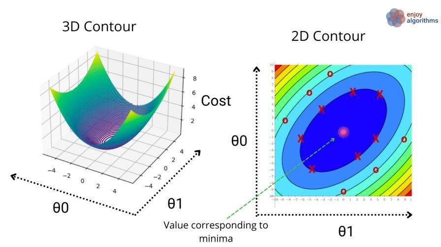
Contour lines are lines on which a function's value remains constant despite variable changes. When the variables (θ1 and θ0) change, the cost function value remains the same along these contour lines.

What is a contour plot?

A contour plot consists of many contour lines, like in the image below.

• In the 2D contour plot, we have oval lines on which the cost function value for all the red-X points will be constant. And in the same manner, the cost function values for all the red-O will be the same.
• If you observe the 3D contour image, the value of the cost function at the innermost centre is the minimum, and if we remember, our objective was to minimize the cost function. The machine will try to reach the pink star position (shown in 2d contour) by trying various values for θ1 and θ0.

Once the machine determines that θ1 = 1 and θ0 = 1 will minimize the cost function, it stores these values as the learned parameters. These learned parameters will then be used for future predictions.

What if there are more than two parameters to learn?

There can be various scenarios where we need to learn many parameters. For advanced deep learning models, the number of parameters to learn can be billions. Let's take one example. Suppose we have to learn a function of this format.

Correlating this with a real-life example, Suppose we want to predict the price of various houses. The cost of a house majorly depends upon the size of the house (2-BHK, 3-BHK, etc.). We need to include other essential factors that affect the price, like location, number of floors, connectivity distance from the railway station and airport, and many more. In that case, the machine must learn parameters for every factor. These parameters will be treated as the weightage of each factor in determining the price of the house.

Let's assume that X1, X2, …, Xm are m such factors that affect the price of the house, and we collected n historical data samples for each factor. In the image below, X1 is not a number but an n-dimensional vector.

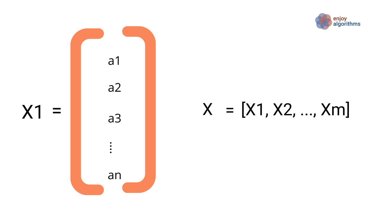
We can represent the equation between input matrix X and output Y as Y = weight.T * X + Bias. Here weight.T is the transpose of the weight matrix. 

For analyzing a single sample, the input matrix X will have dimensions of (1 x m), where m represents the number of parameters or dimensions. Similarly, the Bias matrix will have the same dimensions as the output, which is nothing but the price of that flat. It is (1 x 1) for a single sample.

The product of weight.T * X should result in (1 x 1) dimension to ensure that the addition in the above equation is valid. Since X has dimensions of (m x 1) with all factors represented as a single-column matrix, the weight matrix must have dimensions of (m x 1). If we transpose the weight matrix (weight.T), it will result in a (1 x m) size matrix, allowing the product of weight.T * X to have (1 x 1) dimension ( 1 x m ) * (m x 1) → (1 x 1).

If we consider all samples in one go, the weight matrix will be m X n, as shown below.

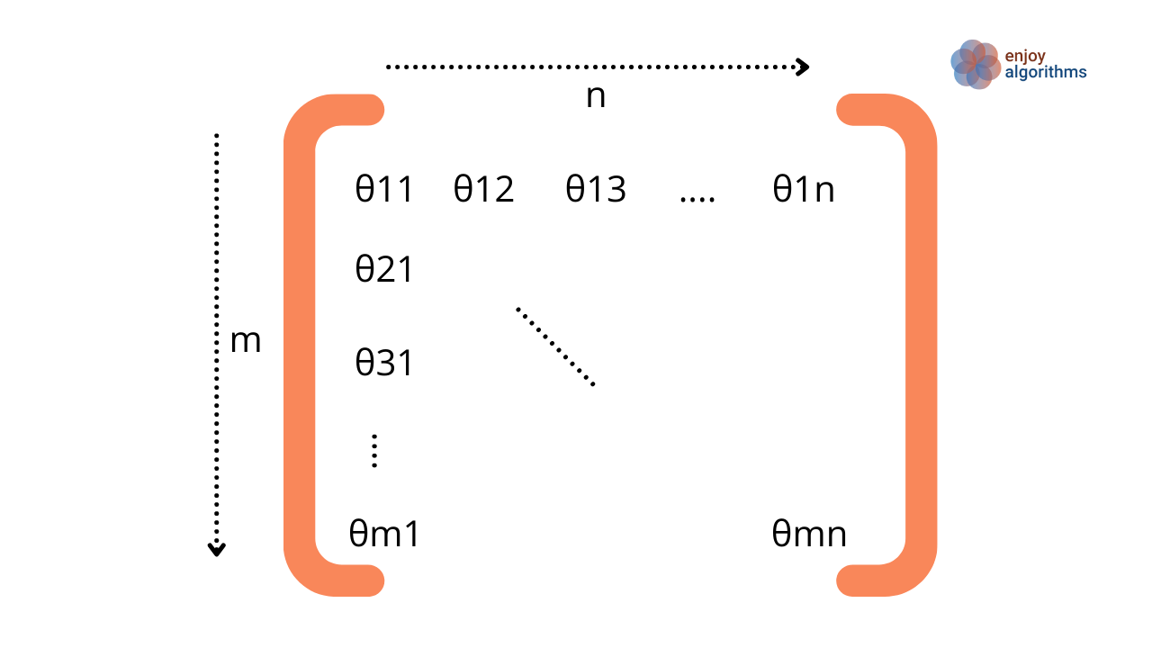
So, machines will learn all these parameters (θ11, θ12, …, θmn) of the weight and the bias matrices.

That's how the machine learns multiple parameters in representing a function.

Possible Interview Questions

In machine learning interviews, interviewers often assess the candidate's foundational knowledge by asking basic concept questions. Some of the most common questions from this article include:

• What is a cost function in machine learning, and why is it defined?
• What are the odds of the machine finding the minimum of the defined cost function if it selects and updates parameters randomly?
• How do machines store and use their learnings for new inputs?
• What happens if the machine doesn't reach the perfect minimum?
• What are contour plots, and how are they used in machine learning?

Conclusion

In this article, we developed a basic intuition behind the cost function involvement in machine learning. We demonstrated machines' step-wise learning process through a simple example and analyzed how machines find suitable values for various parameters and memorize these learnings. We hope you enjoyed the article.