Credit Card Fraud Detection Project Using Machine Learning

As we move toward the digital world, cybersecurity is becoming a critical part of our lives. For example, when we purchase any product online, many customers prefer credit cards as an option. But on another side, credit, debit, and other prepaid card-related fraud activities have been rising these days. The common purpose of these activities is to extract finance-related credentials from individuals and perform financial transactions on their behalf. To handle this problem these days, machine learning algorithms can help us track abnormal transactions, classify them, and stop the transaction process if required.

This article will guide you through the step of detecting such fraudulent transactions performed on credit cards by developing a machine learning model. Several classification algorithms can perform the best and are easily deployable, like support vector machines, logistic regression, etc. We will be using a Random Forest Classifier to build our fraud detector. So let’s start without any further delay.

Implementation Steps using Random Forest Classifier

Step 1: Downloading and loading the dataset

We will be using this standard dataset on Kaggle to demonstrate our steps, starting from exploring the dataset to building a model and finally evaluating the performance on several indexes. Once we have the data, creditcard.csv (150.83 MB), we will use pandas to read the CSV data and obtain a DataFrame to work on.

# import the necessary packages 
import numpy as np 
import pandas as pd 
import matplotlib.pyplot as plt 
import seaborn as sns 
from matplotlib import gridspec 
#####################################

# Load the dataset from the csv file using pandas 
data = pd.read_csv("creditcard.csv")

Step 2: Exploring the dataset

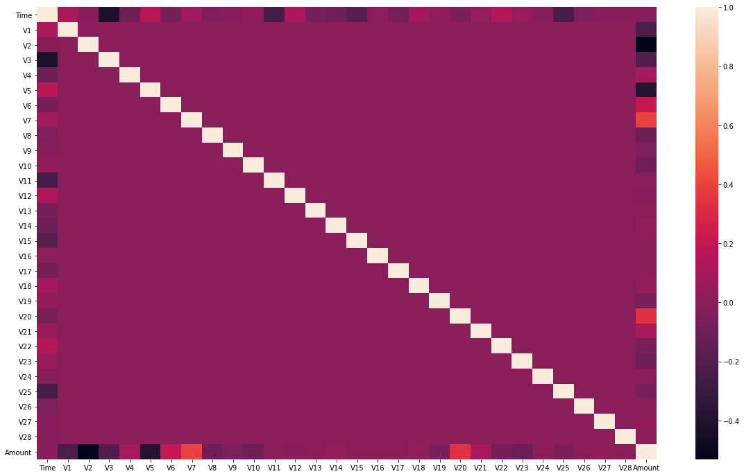
The more we know our data, the more confident we will be about the behavior of our machine learning model. There are various data analysis techniques that we can use to explore our data deeper. One such method is plotting the cross-correlation matrix using the heatmap function of the Seaborn library. We need to check the relationship among input attributes, and hence we will remove the columns corresponding to the target variable and plot the correlation matrix for the rest of the features.

• Heatmap Exploration

# dropping the target column
df_features = data.drop(columns='Class')

# plotting
plt.figure(figsize=(20,12))
sns.heatmap(df_features.corr(), annot=False)
plt.show()

We can infer from the above figure that the features are mostly uncorrelated, which means the variation in one feature very minutely affects variation in another feature.

• Target Variable Distribution Analysis

print(data.shape)
# (284807, 31)

# Fraud and genuine datasamples
fraud = data[data['Class'] == 1]
valid = data[data['Class'] == 0] 

print('Fraud Cases: {}'.format(len(data[data['Class'] == 1]))) 
print('Genuine Transactions: {}'.format(len(data[data['Class'] == 0]))) 

# Fraud Cases: 492
# Genuine Transactions: 284315

The dataset has a total of 284807 instances and 31 features which are divided into two categories of Fraud and Genuine transactions. This is highly unbalanced, with the majority of the cases belonging to genuine transactions.

• Fraud Transactions: 492
• Genuine Transactions: 284315

The above numbers show that more than 99% of the transactions are genuine. Any model trained directly on this data will inherently be biased toward the positive class (genuine transactions or non-fraud transactions). We will manipulate this dataset to make our model unbiased toward any categories. We will build two different models here to demonstrate the effect of unbalanced-ness and show how accounting for this will improve the model's performance.

• tSNE Visualization

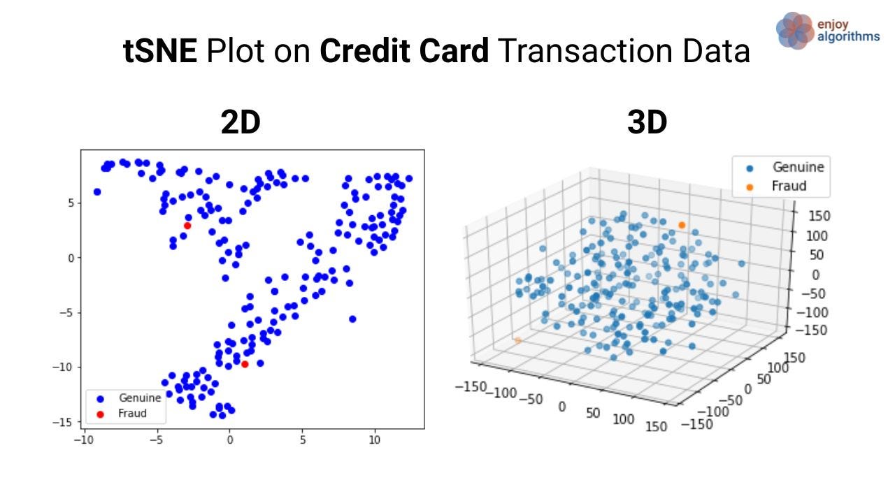
Plotting the entire dataset in the 3D tSNE plot will be time-consuming. Hence we will first make a newer dataset by randomly selecting 500 data samples from the original dataset. The newer dataset will be a subset representative of the original one, and the tSNE on this dataset can be shown in the image below.

from sklearn.mainfold import TSNE
# X will be the subset representative
# Take 200 data points as it's hard to analyze too many points
X = data.drop('Class',axis=1)[280100:280300]
target = data['Class']
y = target[280100:280300]

tsne2 = TSNE(n_components=2, random_state=0)
tsne3 = TSNE(n_components=3, random_state=0)

# 2D plot
X_2d = tsne2.fit_transform(X)
target_ids = range(2)

from matplotlib import pyplot as plt
plt.figure(figsize=(6, 5))
colors =  'b','r', 'c', 'm', 'y', 'k', 'w', 'orange', 'purple'
for i, c, label in zip(target_ids, colors, ['Genuine','Fraud']):
    plt.scatter(X_2d[y == i, 0], X_2d[y == i, 1], c=c, label=label)
plt.legend()
plt.show()

# 3D plot
X_3d = tsne.fit_transform(X)

fig = plt.figure()
ax = fig.add_subplot(111, projection='3d')

n = 200
target_ids = range(3)

colors =  'g','r', 'b', 'c', 'm', 'y', 'k', 'w', 'orange', 'purple'
for i, c, label in zip(target_ids, colors, ['Genuine','Fraud']):
    #plt.scatter(X_2d[y == i, 0], X_2d[y == i, 1],X_2d[y == i, 2], c=c, label=label)
    ax.scatter(X_3d[y == i, 0], X_3d[y == i, 1],X_3d[y == i, 2],label=label)
plt.legend()
plt.show()

Objective flowchart of the problem statement

The above flowchart shows the tasks in sequential order, which we will be executing in this blog. From the previous data analysis step, we know that the data is highly unbiased, and hence we need to perform pre-processing to make it balanced. We will try to cover three sampling techniques to balance the data in this article.

1. Upsample the minority class: Try to increase the data samples, particularly for those with lesser instances in the original data.
2. Downsample the majority class: Try to decrease/drop data samples, particularly for those with higher instances in the original data.
3. SMOTE: Synthetic Minority Over-sampling TEchnique (SMOTE)

Once we make the data balanced, A random forest classifier model will be built for all four cases, and we will analyze the performance for each of these cases. It should be evident from the flowchart that we will not touch the test set to evaluate the model fairly, and every process of sampling should be strictly limited to the training dataset. So, let’s learn about all these techniques using the context of the current problem statement.

Step 3: Data Pre-processing

Let's perform the sampling of data to make it balanced using all three methods mentioned in the flowchart,

Up Sampling

from sklearn.utils import resample

not_fraud = X_tr[X_tr.Class==0]
fraud = X_tr[X_tr.Class==1]

fraud_upsampled = resample(fraud,replace=True,n_samples = len(not_fraud),random_state = 27)

upsampled = pd.concat([not_fraud, fraud_upsampled])

In this process, the minority class, which is the fraudulent type, is up-sampled to match the number of instances in the majority class. The sample size of the dataset is now changed as follows :

It is to be noted that only the training samples are subjected to this pre-processing, which is 75% of the total samples. Upsampling can be done using the utils package from sklearn — from sklearn.utils import resample. We extract the minority class and upsample it as per the number of instances in the majority class, using the resample package.

Down Sampling

from sklearn.utils import resample

not_fraud = data[data.Class==0]
fraud = data[data.Class==1]

not_fraud_downsampled = resample(not_fraud,replace=True,n_samples = len(fraud),random_state = 27)

downsampled = pd.concat([fraud, not_fraud_downsampled])

Similar to upsampling, downsampling can be done using the resample package. Here downsize the majority class as per the size of the minority class.

SMOTE

Machine learning algorithms have trouble learning when one class dominates the other. This dataset is very much relevant to this problem that we are facing. Synthetic Minority Over-sampling TEchnique (SMOTE) is an up-sampling of the minority class and some associated rules. SMOTE synthesizes new minority instances between existing minority instances. Here the up-sampling is done along the trajectory of the path connecting any two minority classes.

In the simplest form, SMOTE generates new samples along the lines connecting the minority class. SMOTE is not in-built in sklearn. So, we will have to download a package called the imbalanced-learn, which can be downloaded using the pip command (Linux:sudo pip3 install imbalanced-learn). Then, the SMOTE class can be imported, and an instance of the same can be created.

from imblearn.over_sampling import SMOTE
over = SMOTE()

This completes our three different pre-processing steps, and now we will move forward to the model building and training phase on the four types of datasets that we formed.

1. Original Dataset (Base case), 2. Upsampled Dataset, 3. Downsampled Dataset, 4. SMOTE Dataset

Step 4: Model Formation

We will build a Random Forest Classifier and train the same for all four different cases in this step. The random forest can be imported from the sklearn library from sklearn.ensemble import RandomForestClassifierand then be used to fit the data. The model will then be evaluated in each of the categories with a detailed classification report.

The Base case is when no form of sampling is done, and the model is directly trained on the dataset.

Base: Training Set: 213605 (75%), Testing Set: 71202(25%)

Note that this testing set will be fixed throughout the evaluation process.

Up Sampling: Training Set: 213605 (75%) → 426472, Testing Set: 71202(25%)

Note that this is the step where the training takes more time than the other methods.

Down Sampling: Training Set: 213605 (75%) → 738, Testing Set: 71202(25%)

Note that this is the step where the training takes a minimum time of all the methods.

SMOTE: Training Set: 213605 (75%), Testing Set: 71202(25%)

# Building the Random Forest Classifier (RANDOM FOREST)
from sklearn.ensemble import RandomForestClassifier

# random forest model creation 
rfcD = RandomForestClassifier()
rfcD.fit(xTrain, yTrain)

# predictions 
yPred = rfcD.predict(xTest)

Step 5: Performance Evaluation

We will use several metrics to show the model’s performance from a different point of view.

# Evaluating the classifier 
# printing every score of the classifier 
# scoring in anything 
from sklearn.metrics import classification_report, accuracy_score 
from sklearn.metrics import precision_score, recall_score 
from sklearn.metrics import f1_score, matthews_corrcoef 
from sklearn.metrics import confusion_matrix 

n_outliers = len(fraud) 
n_errors = (yPred != yTest).sum() 
print("The model used is Random Forest classifier") 

acc = accuracy_score(yTest, yPred) 
print("The accuracy is {}".format(acc)) 

prec = precision_score(yTest, yPred) 
print("The precision is {}".format(prec)) 

rec = recall_score(yTest, yPred) 
print("The recall is {}".format(rec)) 

f1 = f1_score(yTest, yPred) 
print("The F1-Score is {}".format(f1)) 

MCC = matthews_corrcoef(yTest, yPred) 
print("The Matthews correlation coefficient is{}".format(MCC)) 

from sklearn.metrics import roc_auc_score
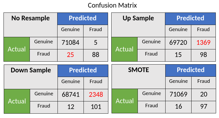
print(roc_auc_score(yTest, yPred))

• Confusion Matrix : This gives us an overall picture of the model performance but does not justify the model’s robustness due to imbalanced data.

For the first case where no sampling is employed, the model performance in Fraud cases is poor, with an error of more than 22%. Employing either Up Sampling or Down Sampling results in more genuine cases being identified as fraudulent cases. The SMOTE resampling provides a trade-off between the two cases.

• Mathew’s Correlation Coefficient : The Matthews correlation coefficient is an attested score that is high only if the prediction obtained superior results in all categories (true positives, false negatives, true negatives, and false positives) of the confusion matrix, proportionally both to the size of the two distinct categories in the dataset.

BASE: 0.858, UPSAMPLING: 0.238, DOWNSAMPLING: 0.188, SMOTE: 0.853

This correlation and the confusion matrix shows how one can achieve better accuracy for actual fraudulent cases (minority cases). Now that we have implemented the credit card fraud detection system, let's see where such techniques are employed in industry-based applications.

Companies Case Studies

Firewall for internet security protecting against identity theft

A good firewall provides security against “identity thieves.” These can be hackers or scammers who can burgle inside vulnerable computer systems and steal private files, credit card information, tax records, passwords, and identification or reference numbers. Skilled hackers can even seize a system to plant destructive computer viruses, or plant another information-stealing agent in our system or send spam messages to target our financial information.

For example, the cyber-criminal knows the victim made a recent purchase at Apple. Then they can send an email disguised to look like it is from Apple customer support. The email tells the victim that their credit card information might have been compromised and confirms their credit card details to protect their account. A firewall can test the electronic data coming in or out of a computer and use a classifier shown above to estimate whether the user is genuine or fraudulent.

Biocatch for identifying scammers

Biocatch is a behavioral biometric solution that designs payment fraud strategies from an individual level to an organizational level that identifies online fraudsters by their actions such as familiarity in the application process, navigation, and data input eCommerce site. Issuers embed this technology onto an application software or website to prevent real-time fraud. It conducts continuous verification by gathering and processing several attributes once the user logs in. The data collected can be sent to an ML pipeline which can provide significant knowledge about the users’ intent.

If one wanna know about more companies, they can explore this link: 11 Companies That Teach Machines To Detect Fraud.

Possible Interview Questions

Interviewers can ask questions based on this machine learning application or similar machine learning projects. Some of them can be:

• What is Random forest, and on what principle does it work?
• What is the ensemble learning approach? Is random forest an ensemble learning algorithm?
• Did you try some different algorithms? Can you justify the benefits of random forest over other algorithms?
• A confusion matrix is the best way to identify a better model. What is a Type 1 or Type 2 error in that?
• For fraud transaction detection, many companies collect users’ private information. Isn’t it making them more vulnerable?

Conclusion

This article presents how machine learning applications can help in securing privacy and protect us from financial loss because of spam and fraud. We built our own random classifier model using the Kaggle dataset and applied different pre-processing over it, including SMOTE. After that, we evaluated our model and justified how pre-processing and balancing out the data is important pre-processing and balancing the data. We also presented the two companies' use-case based on this machine learning project. We hope you have enjoyed the article.

Enjoy Learning, Enjoy Algorithms, Enjoy Machine Learning!