Customer Segmentation using Hierarchical Clustering

What is Customer Segmentation?

Customer segmentation helps businesses develop customer-focused marketing strategies. The reason is simple: Every customer has different choices, so one approach only applies to some customers. So the goal of segmenting customers is to make segment-wise decisions and maximize the value of each customer to the business.

Customer segmentation splits the organization's customer base into smaller groups that reflect similar behaviour. With the current advancements in machine learning and artificial intelligence, this is no longer a challenging task.

What is Clustering?

Clustering is an unsupervised machine learning task that divides data points into groups based on feature similarities and allocates them into clusters. Ideally, the clusters should be distinct and non-overlapping.

Clustering is prevalent in many fields, and there are several clustering algorithms, but for this blog, we will limit ourselves to Hierarchical Clustering.

Let's Understand Customer Segmentation with an Example

Suppose Walmart has collected customer data based on past transactions such as the customer's gender, age, annual income, spending score, and shopped item category. With the availability of all these parameters, Walmart's marketing team has sufficient information to explain customers' spending habits.

Now imagine Walmart is launching a campaign targeting customers interested in luxurious items. They have special offers to attract them to the store, but extending them to all customers will not make sense since not all customers are interested in luxurious items.

We can segregate similar users who can buy luxury items using customer data to address this problem. The problem can be solved using clustering algorithms, where we can cluster the customers into different segments and select the cluster of potential customers for the campaign.

In this blog, we want to explore the potential of clustering algorithms to accomplish the above task. Let's start the clustering analysis.

Clustering Analysis

Our goal is to divide customers into different groups such that customers falling into the same group will share similarities in terms of their spending habits. We will be using Kaggle's Mall Customer Segmentation dataset for the implementation. It's a small dataset having 200 customers' data and spending scores.

import pandas as pd
customer_data = pd.read_csv('Mall_Customers.csv')
customer_data.head()

#####################################################
'''
      customerID |  Gender  | Age | Annual Income (k$) | Spending Score
   0      1      |   Male   | 19  |       15           |      39
   1      2      |   Male   | 21  |       15           |      81
   2      3      |   Female | 20  |       16           |      6 
   3      4      |   Female | 23  |       16           |      77
   4      5      |   Female | 31  |       17           |      40       


'''
#######################################################

We have four columns of concern and one Customer ID column. Each row in this dataset represents a customer. We have the age, gender, customer's annual income, and spending score for each customer.

Hierarchical Clustering

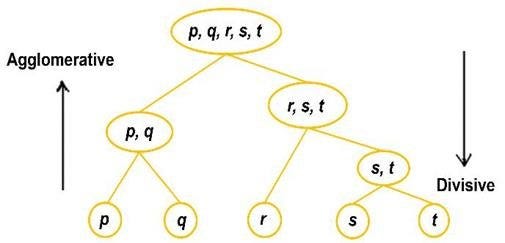
Hierarchical Clustering is an unsupervised machine-learning algorithm that groups similar objects into groups called clusters by creating a hierarchy of nested clusters. The outcome of this algorithm is a set of clusters where data points of the same cluster share similarities. Furthermore, the Clustering can be interpreted using a dendrogram.

Hierarchical Clustering has two variants:

• Agglomerative hierarchical clustering
• Divisive Hierarchical clustering

Agglomerative hierarchical clustering

Agglomerative hierarchical clustering is the commonly used approach where we start with individual clusters for each data point and merge them based on their closeness. The final cluster contains all the data points.

In other words, this clustering starts with each data point as a separate cluster and then progressively merges the most similar clusters until a single cluster containing all the data points is formed.

Divisive Hierarchical clustering

Divisive is quite the opposite of the Agglomerative approach. Here, we start with a single cluster containing all the data points. At each step, we split the most distant data point in the cluster, and this process is repeated till we arrive at the individual data points.

For the customer segmentation problem, let's stick with the agglomerative approach since it is commonly used across industries. Now the critical question is: What are the criteria for calculating the nearness or closeness of two clusters? This is where the Proximity Matrix comes into the picture. Let's understand the concept of the Proximity Matrix using a small example.

Imagine we have the monthly salaries of five working professionals, and we want to group similar professionals based on their monthly salaries. Here, we will use hierarchical clustering to group similar professionals together.

salary id   |   salary
   1        |    2000$
   2        |    5500$
   3        |    4000$
   4        |    4500$
   5        |    2500$

Firstly, we need to create a proximity matrix, which is a square matrix of n x n dimensions containing the Euclidean Distances. If you need to learn about Euclidean distance, here's a quick link. The Euclidean distance formula is defined as follows:

Let's take a look at the proximity matrix:

Proximity Matrix is also known as the Euclidean Distance Matrix.

The distance between self is zero, so the proximity matrix's diagonals are always zero. We will merge the professionals with the lowest distance in the proximity matrix for pairing similar professionals. The minimum distance is 500 per the above proximity matrix, not to be confused with zero, the distance with self. So, professionals 1 and 5 can be paired into one cluster, and professionals 4 and 3 can be paired into another cluster since the Euclidean distance is Lowest.

Clusters formed: (1, 5) and (3, 4).

We will repeat the above process in the next iteration by constructing another proximity matrix. Before that, let's update the salary table. Note: After making a cluster, we need to specify the criteria for assigning a salary to the so-formed cluster. Here, we are using the maximum function. Some other options are minimum and average.

   Clusters    |    salary
     (1,5)     |     2500$
       2       |     5500$
     (3,4)     |     4500$  

Let's build the proximity matrix:

Here, we can see (3, 4) cluster shares similarities with professional 2 since their distance is lowest. Time to group them to update the clusters.

Clusters Formed: (1, 5) and (2, 3, 4).

Now, we are left with only two clusters; this time, whatever distance value comes up in the proximity matrix, these clusters are bound to merge. The final cluster will contain all the professionals.

Let's finally conclude the Clustering formed in this case using a Dendrogram.

What is Dendrogram?

A dendrogram is a visual representation of the hierarchical relationship between clusters. The X-axis contains the samples, also known as the leaf nodes, and Y-axis includes the distance between the two clusters or samples. The longer the distance between two samples, the less similar they are, and the converse is true. Following is a rough dendrogram of the above example.

To choose the number of clusters, we locate the most extensive vertical line, and we usually draw a horizontal line cutting the most extensive vertical line. The y-axis intersection value is the threshold for finalizing the optimal number of clusters. This way is inefficient and depends on the distance between two clusters.

Number of optimal clusters for data = 2.

Python Implementation of Customer Segmentation Using Hierarchical Clustering

Let's apply Hierarchical Clustering to our Customer Segmentation problem. Just before that, we only need to keep the relevant columns.

features = customer_data.iloc[:, 1:4]
features.head()

######################################
'''
       Age | Annual Income (k$) | Spending Score
   0   19  |       15           |      39
   1   21  |       15           |      81
   2   20  |       16           |      6 
   3   23  |       16           |      77
   4   31  |       17           |      40   


'''

#####################################

Features

import scipy.cluster.hierarchy as sch

dendrogram = sch.dendrogram(sch.linkage(features, method = 'ward'))
plt.title('Dendrogam', fontsize = 20)
plt.xlabel('Customers')
plt.ylabel('Ecuclidean Distance')
plt.show()

Dendrogram plotting

Three seems a suitable threshold as per the rule for cutting the most extensive vertical line for finalizing the optimal number of clusters. 

plt.title("Dendrograms")  
dend = shc.dendrogram(shc.linkage(features, method='ward'))
plt.axhline(y=300, color='r', linestyle='--')

Dendrogram cutting on real dataset

The number of optimal clusters is 3. Let's visualize the clusters!

from sklearn.cluster import AgglomerativeClustering
cluster = AgglomerativeClustering(n_clusters=3, affinity='euclidean', linkage='ward')  
cluster.fit_predict(features)

plt.figure(figsize=(10, 7))  
plt.scatter(features['Annual Income (k$)'], features['Spending Score (1-100)'], c=cluster.labels_)
plt.xlabel("Annual Income", fontsize = 15)
plt.ylabel("Spending Score", fontsize = 15)

Clusters at n = 3.

The number of optimal clusters formed according to the rule needs to be more accurate in this analysis. Better rely on intuition and domain knowledge for deciding the optimal number of clusters. In the above plot, we can confirm the presence of 4 clusters. Let's set the optimal clusters as 4 and visualize the position of clusters.

Clusters at n = 4.

This is an excellent improvement in the visualization of clusters. Sometimes, the rule returns misleading information, but we should always confirm the results based on our intuition and domain knowledge.

Going back to the problem statement, after analyzing the above scatter plot, we are interested in the red-coloured cluster because these customers have a high annual income and a high spending score, which is precisely what we are looking for.

Now, we can hand over these customers to the marketing team. They will approach these customers with some planned offers, and since they belong to a common cluster, we can confidently say that most customers will respond similarly to the offers.

Advantages of Hierarchical Clustering

• Easy to implement and gives good results in some cases.
• Unlike the K-means clustering algorithm, Hierarchical Clustering does not require the user to define the number of clusters (represented by K) before running the algorithm.

Disadvantages of Hierarchical Clustering

• The execution time for Hierarchical Clustering can be pretty high. Because the algorithm creates a hierarchy of nested clusters by iteratively merging or splitting clusters, the computational complexity can increase rapidly with larger datasets.
• It can be hard to determine the accurate number of clusters using the dendrogram. In other words, the dendrogram can be useful for visualizing the relationships between clusters, but it can be challenging to identify the optimal number of clusters based on the dendrogram alone. This requires the user to interpret the dendrogram based on domain knowledge and intuition, which can be subjective and prone to error.

Due to its high time complexity, using hierarchical Clustering over a Million Row Dataset is out of the question. Hence, it is not preferred for large to medium-range datasets.

Conclusion 

We began with a brief introduction to the customer segmentation problem and discussed the workings of Hierarchical Clustering using a small example. We also spent some time understanding the proximity matrix and dendrograms.

Finally, we implemented Hierarchical Clustering on our customer segmentation dataset and visualized the results using the dendrogram and scatterplot. We concluded with the implementation, followed by a discussion of the pros and cons of the Hierarchical Clustering algorithm.

If you have any queries/doubts/feedback, please write us at contact@enjoyalgorithms.com. Enjoy learning, Enjoy algorithms!