Decision Tree: A Tree-based Algorithm in Machine Learning

Introduction

Trees have a very close connection with almost every Computer Science domain, and Machine Learning is not an exception here. We might be aware of the flowcharts that we use to make decisions. For example, if the atmospheric temperature is < 15, take a bath, otherwise not. In the same way, industry experts try to form some business decision rules using tree-like flowcharts. Using Machine Learning, we try to automate this formation of the flowchart, which will be later used for predictions or taking decisions. The decision tree is one such algorithm.

A Decision Tree is a hierarchical breakdown of a dataset from the root node to the leaf node based on the governing attributes to solve a classification or regression problem. Decision Trees (DTs) are a non-parametric supervised learning algorithm that predicts the value of a target variable by learning rules inferred from the data features.

But before moving any further, let's first learn some basic terminologies of tree-based algorithms.

• Root Node: The top of the tree contains the most essential attribute for the training data.
• Splitting: Divison of nodes into two or more sub-nodes.
• Branch Node: If the sub-node is further split. Each condition is represented as the branch node and is also known as a decision node.
• Leaf Node: Nodes that do not split are the leaf or terminal nodes.
• Parent node: If the node is split into sub-nodes, that node is the parent for the sub-nodes formed after splitting.
• Child node: All the sub-nodes of the parent node.
• Pruning: Removing some splitting, we can consider this as the opposite of spitting.

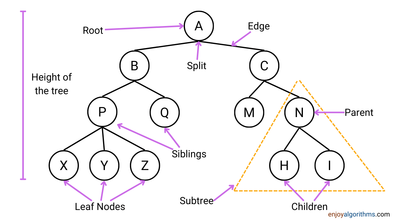
Now, as we know the terminologies, it will be easier to follow the theory. To get better hands-on, let's take a very popular dataset of PlayTennis and follow the formation of a flowchart. Here the objective of this flowchart would be to decide whether tennis play will happen or not based on the outlook, temperature, humidity, and wind conditions.

Dataset Example

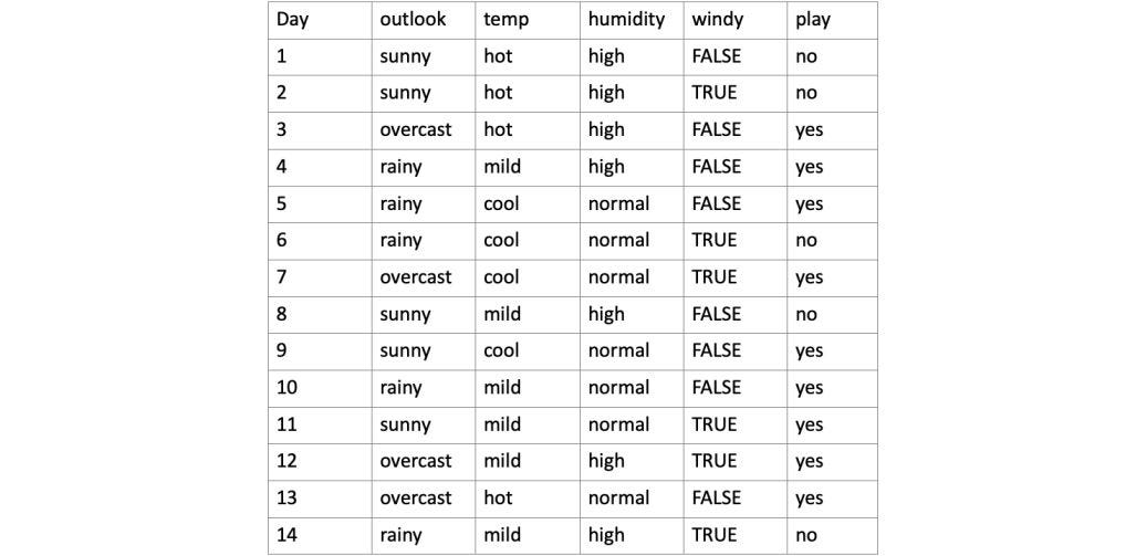
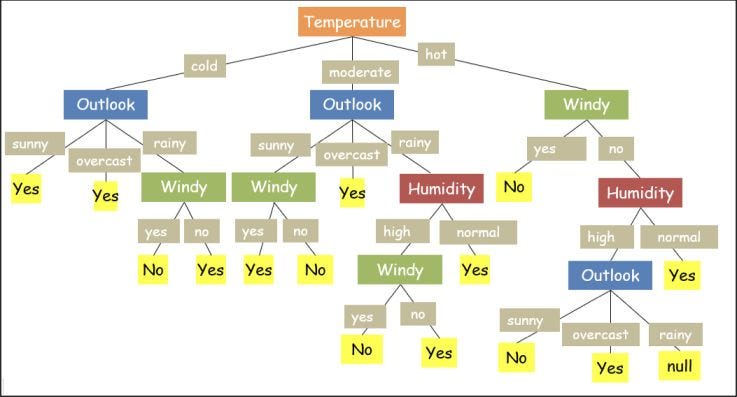
A decision tree is a visualization of attributes governing the decision hierarchically. Consider the dataset above. Fig.1 shows one of the possible decision trees for the given dataset. If we notice carefully, some attributes (such as temperature) in the dataset are redundant, i.e., the decision is independent of that particular attribute.

If we closely examine another possible tree for the same example above, shown in Fig.2, the output of this tree will be the same as the previous one; however, this tree is somewhat lengthy (more nodes from root to leaf). But flowchart with a lesser number of nodes appears to be more clearer. Hence, we prefer "smaller trees" whenever possible for a decision tree.

There is still a big puzzle for us: How do we decide which attribute/feature will give us the smaller tree? To decide the best attribute, which will give us a smaller and better flowchart, we calculate the Information Gain for every attribute, which depends on the term entropy. So, let's first learn about these concepts.

Entropy

In our loss function's blog, we learned about this term. Let's quickly revise it here. The Entropy of a dataset is the average amount of information needed to classify any observation in the data. It is termed Uncertainty. If Entropy is higher, the confidence in classifying any observation into any class is lower and vice-versa.

For an equally balanced categorical value, the Entropy is equal to 1. A real-world dataset may not necessarily be balanced. In the given example, the output cases (yes & no) are imbalanced, i.e. [9 'yes' and 5' no'], so the Entropy is not equal to 1.

Information Gain

Any attribute chosen to partition a tree will result in a loss of Entropy. This means that on choosing any attribute to form a tree, the balancedness of the dataset will reduce. Information gain is the measure of the effectiveness of an attribute in retaining the Entropy. The attribute with the highest information gain is chosen as the next node (first in the case of "root node") in the tree.

In the above equation, Sv/S is the probability of that particular value in the given data. If it's difficult to understand, wait for a while, and it will get easier.

Let's take the example of an ID3 Decision tree and build it from scratch. ID3 stands for Iterative (iteratively) Dichotomizes (divides) the dataset into two or more sub-groups. It is inherently a greedy approach, which means it always selects the best attribute to perform the splitting. 

Pseudo Code for building an ID3 decision tree.
Main Loop:
  if (all the observations belong to the same target class):
       then output is a leaf node with that class
  else:
       A <-- [the "best" decision attribute for next node]
       Assign A as the decision attribute for node
       For each value of A, create new descendant of node
       
       Sort training examples to descendant nodes
       
       If training examples are perfectly classified, then STOP,
       else iterate over new child nodes.
       Attributes that have been incorporated higher in the tree 
       are excluded, which means any given attribute can appear 
       only once in any particular level of the tree.
  best attribute:
       the attribute with the highest information gain (I.G.),
       w.r.t. the parent node, is termed as the best attribute

ID3 decision-tree implementation (Numerical calculations and with code in python)

The example is taken from the Machine Learning Book by Tom Mitchell. We will build the tree step by step, demonstrating the mathematical calculations and code representing it.

Two libraries — numpy and pandas, are imported for algebraic operations and creating the dataframe, respectively. Calling the function importdata( ) will give the table T(1), the dataset used to demonstrate the working of the ID3 decision tree.

import numpy as np 
import pandas as pd
def importdata(path = 'D: /EnjoyAlgorithm/PlayTennis.csv'):
  data = pd.read_csv(path, header = 0, skiprows = 0)
  
  print("Dataset Length: ", len(data))
  print ("Dataset Shape: ", data. shape)
  
  data.target = data['play']
  return data

First, we check the Entropy of the dataset using (1). There are two different classes in the output, so c = 2. Next, among the 14 samples of the dataset, 9 are 'yes' and 5 are 'no'. Thus:

Due to an imbalance in the dataset, the Entropy is not equal to 1. The function written below can compute the Entropy of the entire dataset or the dataset with respect to any particular attribute.

#Entropy(data) Entropy(data.Loc[data['outlook']=='sunny'])

def Entropy(data):
  
  d = data.iloc[:,-1]
  d = d.value_counts()
  s = 0
  for v in d.keys():
    p = d[v]/sum(d)
    s -= p*np.log2(p)
  return(s)

For example:

With respect to the above Entropy, we can compute the Information Gain for each attribute separately using (2):

Let's first calculate the IG of the "Outlook" attribute.

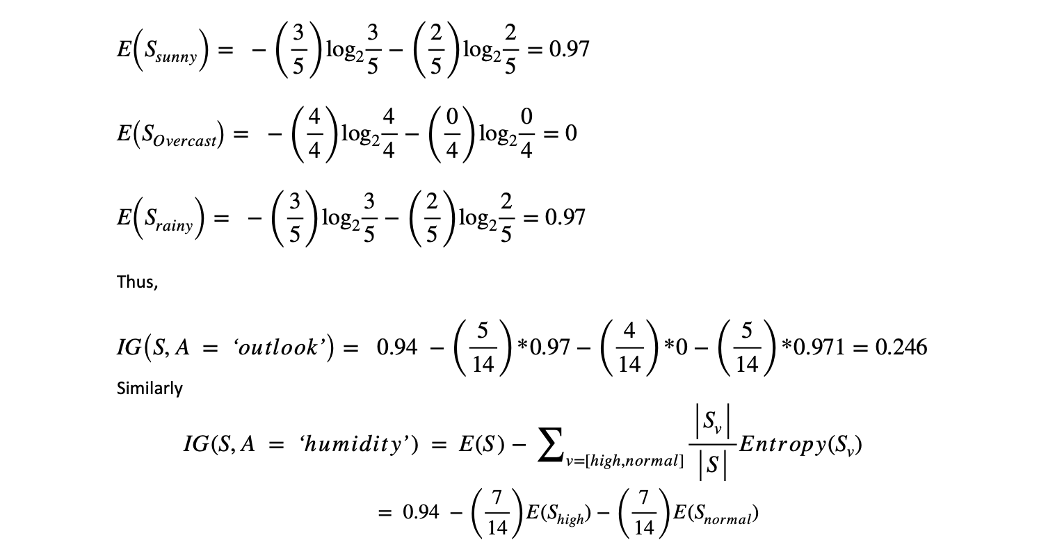
The code below can compute the information gain with respect to any attribute's Entropy value.

def values(attr):
    l = []
    for x in attr:
       if x not in l:
          l.append(x)
    return l

'''
values(data)
['outlook', 'temp', 'humidity','windy', 'play']
values(data['outlook'])
['sunny','overcast','rainy']

'''

The function values( ) is a helper function that can be used to list down the unique values present in the attribute names of any entity.

def IG(data,A): #IG(data, 'outlook')

	Es = Entropy(data)
	val = values(data[A])
	s_c = data[A].value_counts() 
	s_v = []

	for v in range(len(val)):
		ds = data[data[A] == val[v]]
		s = 0; 
		for res in values(data.iloc[:,-1]): 
			try:
				pi = ds.iloc[:, -1].value_counts()[res]/len(ds)
				s -= pi*np.log2(pi) 
			except:
				s = 0 
		s_v.append(s)

	for i in range (len(val)):
		Es = Es - s_c[val[i]]*s_v[i]/sum(s_c) 

	return Es

Using the function above, the IG of the dataset regarding the remaining attributes ('windy' & 'temp') is calculated.

By comparing the information gain of all the attributes of the dataset ([‘outlook = 0.246’, ‘temp = 0.029’, ‘humidity = 0.152’, ‘windy = 0.048’]), it is observed that ‘outlook’ has the highest information gain, IG(S, A = ‘outlook’) = 0.246. Thus, the first node is selected as 'outlook'. 

The tree so far:

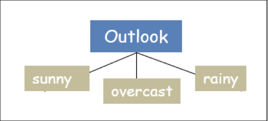
Now concerning each attribute of outlook (['sunny',' overcast',' rainy']), the information gain is to be computed for all the remaining attributes of the dataset (['humidity', 'temp', 'windy']), provided the Entropy of the dataset is not zero. Please remember that every attribute can appear only once in the tree. Now let's further grow the tree.

Outlook — Sunny:

The Entropy of the dataset is non-zero, so information gain is computed.

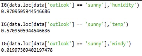
Thus, the following attribute with respect to 'sunny' to be chosen is 'humidity', as it has the highest information gain with respect to the decision question 'sunny.'

Outlook — Rainy:

The Entropy of the dataset is non-zero, so information gain is computed.

Outlook — Overcast:

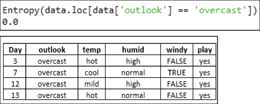
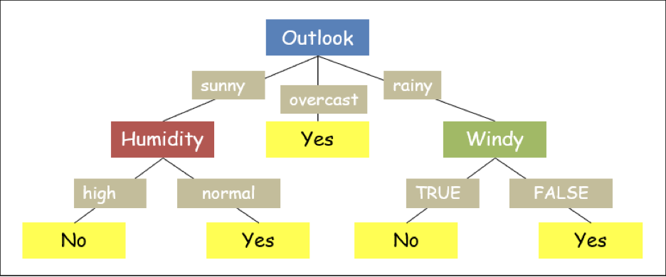
Now, with respect to 'overcast', the Entropy of the dataset is 0. This means that all the observations with respect to this attribute have the same class ('yes' in our case). Thus, the output can be labeled 'yes' for the 'overcast' attribute of 'outlook'. Thus, the tree further grows as:

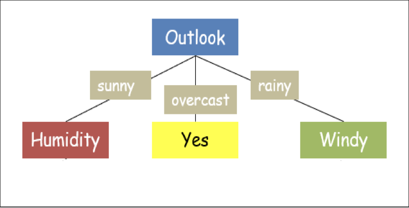
The remaining (unused) attribute of the dataset is 'temp'; thus, the IG needs to be computed with respect to 'humidity' and 'windy'. 'Humidity' has two attributes — 'high' and 'normal', and it has 'overcast' with the decision 'sunny' as its root (parent) node.

Outlook — sunny — Humidity — high:

As the Entropy of the above dataset is 0 thus, the output can be labeled as the only class present in the dataset ('no') for the attribute 'high' of 'humidity' along the tree.

Outlook — sunny — Humidity — normal:

As the Entropy of the above dataset is 0 thus, the output can be labeled as the only class present in the dataset ('yes') for the attribute 'high' of 'humidity' along the tree.

Outlook — rainy — Windy — FALSE:

As the Entropy of the above dataset is 0 thus, the output can be labeled as the only class present in the dataset ('yes') for the attribute 'FALSE' of 'windy' along the tree.

Outlook — rainy — Windy — TRUE:

As the Entropy of the above dataset is 0 thus, the output can be labeled as the only class present in the dataset ('no') for the attribute 'TRUE' of 'windy' along the tree. Thus, the final tree can be drawn as:

We are placing the complete code in one place.

import numpy as np 
import pandas as pd

def importdata(path = 'D: /EnjoyAlgorithm/PlayTennis.csv'):

	data = pd.read_csv(path, header = 0, skiprows = 0)

	print ("Dataset Length: ", len(data))
	print ("Dataset Shape: ", data. shape)

	data.target = data['play']

	return data

def Entropy(data): #Entropy(data) Entropy(data. Loc[data['outlook']=='sunny'])

	d = data.iloc[:,-1]
	d = d.value_counts()
	s = 0 

	for v in d.keys():

		p = d[v]/sum(d)
		s -= p*np.log2(p)

	return(s)



def IG(data,A): #IG(data, 'outlook')

	Es = Entropy(data)
	val = values(data[A])
	s_c = data[A].value_counts() 
	s_v = []

	for v in range(len(val)):
		ds = data[data[A] == val[v]]
		s = 0; 
		for res in values(data.iloc[:,-1]): 
			try:
				pi = ds.iloc[:, -1].value_counts()[res]/len(ds)
				s -= pi*np.log2(pi) 
			except:
				s = 0 
		s_v.append(s)

	for i in range (len(val)):
		Es = Es - s_c[val[i]]*s_v[i]/sum(s_c) 

	return Es



class Node():

	def __init__(self,name = None, attr=None):
		self.name = name
		self.attr = attr 

	def call_(self):
		return self.name

def DTNode(data, features_used):
	node = Node()
	IGmax = 0; vbest = None 
	val_list = [v for v in values(data)[:-1] if v not in features_used]

	if val_list != []:

		for v in val_list:

			if IG(data,v) > IGmax:
				IGmax = IG(data,v)
				v_best = v

		if v_best:

			features_used.append(v_best)
			node.name = v_best 
			node.attr = values(data[v_best])

			return (node)
		else:
			return (None)

	return (None)

def DTClassifier(data, features_used):

	root = DTNode(data, features_used)

	DT_dict = {}

	if root != None:
		item = []
		for attr in root.attr:
			dataN = data[data[root.name] == attr]
			if Entropy(dataN) == 0:
				item.append((attr,values(dataN.iloc[:,-1])[0]))
			else:
				dt = DTClassifier(dataN, features_used)
				item.append((attr,dt))

		DT_dict[root.name] = item 

	return (DT_dict)

The decision tree explained above is popularly known as the ID3 decision tree. However, one important thing to note is that the decision tree implemented in the Scikit-learn framework (sklearn.tree.DecisionTreeClassifier) is not an ID3 decision tree classifier. This classifier is a highly robust decision tree model capable of classifying every node based on the training data it has encountered so far. 

Let's implement the tree using Scikit-learn on the same dataset.

Implementing Decision Tree using Scikit-Learn

Step 1: Importing Libraries

Importing the necessary libraries like numpy and pandas, like before, and importing the DecisionTreeClassifier from sklearn.tree to implement the decision tree and use label encoder to form numerical data values from labels. Finally, use Graphviz to plot the tree.

import numpy as np
from sklearn.tree import DecisionTreeClassifier
from sklearn.tree import export_graphviz

import pandas as pd
from sklearn.preprocessing import LabelEncoder
import graphviz

Step 2: Creating a data-frame using the play tennis data

def importdata(path = 'D: /EnjoyAlgorithm/PlayTennis.csv'):

    data = pd.read_csv(path, header = 0, skiprows = 0)
    print ("Dataset Length: ", len(data))
    print ("Dataset Shape: ", data. shape)
    #data.target = data['play']
    
    return data
    
playtennis_data = importdata()

Step 3: Label Encoding

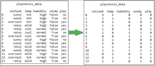
We know that the Machine is unable to understand text features. So, forming a data encoder to convert text-based attributes to numbers. 

#creating a Label encoder to convert text to numbers 
Le = LabelEncoder()
playtennis_data['outlook'] = Le.fit_transform(playtennis_data['outlook']) 
playtennis_data['temp'] = Le.fit_transform(playtennis_data['temp '])
playtennis_data['humidity'] = Le.fit_transform(playtennis_data['humidity'])
playtennis_data['windy'] = Le.fit_transform(playtennis_data['windy'])
playtennis_data['play'] = Le.fit_transform(playtennis_data['play'])

X = playtennis_data[['outlook', 'temp', 'humidity', 'windy']] 
y = playtennis_data['play']

The above operation will change the data as shown below. Every type of attribute is assigned a number which is an integer value.

Step 4: Model Building

Creating a decision tree model fitting the tree with the data that has been generated using the playtennis_data.

X = playtennis_data[['outlook','temp','humidity','windy']]
y = playtennins_data['play']

# create the classifier and train it
tree = DecisionTreeClassifier(criterion='entropy', random_state=0)
tree.fit(X,y)

This will fit the tree on our training data.

Step 5: Plotting the graph using Graphviz

dot_data = export_graphviz(tree, out_file=None)
graph = graphviz.Source(dot_data)
graph.render("iris")

dot_data = export_graphviz(tree, out_file=None, feature_names=
       ['outlook','temp','windy','humidity'], class_names=
       ['no','yes'], filled=True, rounded=True, 
       special_characters=True)
graph = graphviz.Source(dot_data)

graph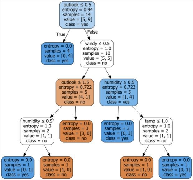

As seen in this decision tree, a classification operation is happening at every node. Some attributes are allowed to occur multiple times at different levels in the decision-making process.

Decision Tree for Regression

The above problem we saw was a classification problem. But decision trees are also capable of solving regression problems as well. We know that the cost function used for solving a regression problem looks like this:

And in the decision tree, we aim to select the attribute which corresponds to maximum information gain or retains the maximum Entropy. In a regression problem, we measure the Entropy of any attribute using the same formulae as above, but in place of the predicted values, we use the mean value of that particular attribute. The attribute with the least cost will be selected for the first candidate attribute to split the data. This same thing can be done with the standard deviation as well.

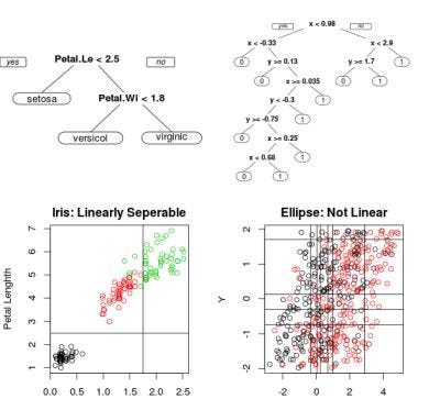
There should be one question coming to our mind: How deep a tree should be grown? This is a tough challenge for the Decision Tree algorithm. Data having a wider set of features often involve more splitting, and the tree becomes very dense. If we go on splitting the nodes for an infinite depth, we will end up in the case of overfitting. Think how?

Because, for every output, we will try to attain perfection by splitting the node further. And eventually, for any unseen data, the model will try to place our test data features into some category that it has seen during training. But it's a kind of possibility that the training set and test set do not match with 100% perfection. To cure this, we apply mainly two solutions:

• Apply conditions on node selection: If the number of samples involved in that step is more than n, only preserve that splitting. 
• Pruning: Remove branches that are created after splitting lesser important features. The most intuitive way of pruning is to start removing leaves till the accuracy of our decision tree deteriorates within the permissible range. This process is commonly known as reduced error pruning. Another method could be to remove such branches which go deeper. This process is called the weakest-link pruning.

Issues in Decision Tree

• How deeply should the tree be grown? : This question becomes a headache, and the perfect answer to this question does not exist.
• How to reduce overfitting? There are methods like pruning and tree-stopping, but they still fail to cover the pervasive but unseen scenarios.
• How to incorporate more training data into an already built decision tree? : This is also another challenge. The addition of data can change the entropy values for any attribute, and the entire tree structure can change. That makes it a perfect non-parametric algorithm in Machine Learning.

Possible Interview Question

DTs are one of the widely known algorithms in the Machine Learning and Data Science domain. Because of many limitations and drawbacks, we generally don't see these algorithms very frequently in resumes. But if one has mentioned this algo in their resumes, possible questions that could be asked from them are:

• What are DTs?
• What are the suffering reasons for this algorithm, and what are the possible ways to cure those sufferings?
• What is pruning, and how does it cure overfitting?
• What is Information Gain, and how does it help find the vital attribute?
• How do we calculate the most important feature in a regression problem?

Conclusion

• A tree has two primary components — node and branch. The node is an attribute for a decision tree, and branches are the decision questions that the nodes use to form the tree further.
• Decision trees classify instances by sorting them down from the root tree to some leaf node. Each node specifies a test of some attribute of the instance. Each branch from the node corresponds to one of the possible values of this attribute.
• An instance is classified by starting at the tree's root node, testing the attribute specified by this node, then moving down the tree branch corresponding to the attribute's value in the given example. This process is repeated for the subtree rooted at the new node.
• Decision trees are convenient for simple classification problems, specifically if the output is a discrete set of categorical values.

References

• Scikit-learn: Machine Learning in Python, Pedregosa et al., JMLR 12, pp. 2825–2830, 2011
• Mitchell, T. M. (1997). Machine learning., McGraw Hill series in computer science New York: McGraw-Hill.

Enjoy learning, Enjoy algorithms!