Forecasting Stock Market Price Using Neural Networks

Introduction

Stock Market is a trading hub where one can purchase shares of companies. Companies use it to raise funds, and stock traders use it to make a profit while trading. Stock traders depend on predicting the future value of stock prices to gain profit, known as the stock market price prediction. Large firms such as Tower Research use statistical models and neural networks to forecast future stock prices to earn profit. This stock market price prediction depends on various factors, such as the past scenarios of the stock market and company performance. In this blog, we will learn how to use ANN on historical data of stock prices to predict future prices.

Key Take Aways From This Article

• Types of stock market price predictions
• Datasets used to predict stock prices and the basics of ANN
• Steps to predict stock prices using ANN
• Comparison of performance of ANN and SVM models
• How companies use ML models to predict future prices and Real-Life fun facts

Types of Stock Market Price Predictions

The stock market price prediction can be broadly classified into three categories depending on the usage, the dataset used, and the technology involved.

• Fundamental Analysis: Fundamental analysis is based on the principle that a company's performance directly affects its stock prices. The data, like the company's reputation and vision for the future, play a key role.
• Technical Analysis (charting): Technical analysis is an investment method used to identify trading opportunities based on patterns of historical trading price and trading volume. 
• Technological methods: The revolution in the capabilities of AI, paired with the advancements in the computer hardware industry, led to support the power-hungry AI efficiently. It has led to a boom in replacing manual analysis with a highly accurate and quicker analysis done by ML models explicitly trained for the task.

In this article, we will be exploring the technological method to support stock trading. But where to get the required data? Let's see some of the most common stock market price prediction datasets.

Datasets available for Stock Market Price Prediction

Some of the popular datasets available online are:

• Historical Stock Market Dataset: This dataset includes historical daily prices for US stocks on NASDAQ and NYSE. The last data was updated on November 10th, 2017.
• Istanbul Stock Exchange: This data was created from finance.yahoo.com and imkb.gov.tr and includes information from the Istanbul stock exchange national 100 indexes, S&P 500.
• Yahoo Finance: This historical data contains the opening and closing price of the market, highest and lowest points and Volume traded for multiple companies like Google, Yahoo, Amazon etc. 
  The yfinance library helps us download the dataset as required. In this blog, we will use this dataset to train our model for Amazon's stock price prediction.

The dataset is acquired, and all that remains now is training an ANN model. Seems easy enough, right? But that is not the case. It follows a series of steps which will be discussed in the coming sections. Let's quickly brush up on the theories about the ANN algorithm behind the model.

ANN (Artificial Neural Network) Basics

ANN stands for Artificial Neural Network. It is an architecture which mimics a human brain and is often used for forecasting tasks. Typically the layers of any ANN model can be classified into three different types; an input layer, a hidden layer and an output layer. 

The input layer, as the name signifies, is the layer which takes features of our dataset as input for training the model, whereas the output layer helps us in getting the required output. The hidden layers are layers between the input and output layers that take the previous layer's output as input, perform mathematical operations and provide it as input to the next layer.The number of hidden layers can vary from 0 to n. Here n can only be an integer value which normally varies from 0–2 and 3–5 for complex datasets. The picture below shows a typical ANN with only one hidden layer.

For our use case, the input feature consists of Adjacent(Adj) close prices of previous days, and the output is the predicted Adj close price for today.
Adjacent close price is a feature in our dataset that is more relevant when compared to the closing price. It is explained in detail in the upcoming section.

Like any algorithmic model, ANN also has its own set of hyperparameters which need to be tuned by us to increase the model's accuracy. We have the following primary hyperparameters →

• The number of hidden layers
• The number of nodes in each layer
• Selection of activation function
• Suitable loss function
• Suitable Optimizer

These hyperparameters are tuned based on experimentation, intuition and academic exploration done by us. 

But have you ever wondered why we need a hidden layer?

The reason is that if there are zero hidden layers, ANN acts like a linear separator, which is suitable for simple classification problems. But generally, ML solutions are required to learn complex patterns, and the output classes are not linearly separable. We add this non-linearity by adding hidden layers and suitable activation functions.

But why many and not just one sufficiently large hidden layer?
This issue hangs on the word "sufficiently large", which is not always practical. A single hidden layer might be optimal for some applications, whereas for many, multi-hidden layers might outperform.

More about ANN can be read in this blog. Let's see the steps for designing a model for stock market price prediction, which includes everything from dataset analysis to model evaluation.

Problem Statement 

Having learnt about the dataset and the underlying concepts of ANN, let's put them to use to achieve our end goal. Shall we revisit the end goal once, but this time in a more technical way?

“Predict the closing price of a particular stock using the historically available prices of the said stock, i.e. given the previous 15 days’ closing price, try and predict the 16th-day closing price”

This is done as previous prices affect the future price, so the latest historical data is considered for the prediction. 

All of us must be curious about the number of days selected as well as why only the stock’s closing price is considered. These all will be discussed in the upcoming sections.

Steps to Implement ANN for Stock Price Prediction

Data Analysis

Data is downloaded from the Yahoo finance dataset using the yfinance library. It consists of Amazon's stock prices for a timeframe of 1 year from the current date. The code is shown below.

import pandas as pd
import numpy as np
from pandas_datareader.data import DataReader
import yfinance as yf
from pandas_datareader import data as pdr
yf.pdr_override()

from datetime import datetime
end = datetime.now()
start = datetime(end.year - 1, end.month, end.day)
AMAZON = yf.download("AMZN", start, end)

The sample records are as shown below →

Let's understand the meaning of each column here →

• Open → This tells us the stock's opening price for a particular day.
• Close → It refers to the stock's closing price for a specific date.
• High → It indicates the highest price of the stock for a day.
• Low → This tells us the stock's lowest price for a day.
• Volume → This depicts the number of Amazon's shares traded in a day.
• Adj(Adjacent) Close → It also refers to the closing price but is a more accurate measure of the stock's value as it considers other factors such as dividends. 

The total length of the dataset is 250, even though there are 365 days in a year. This discrepancy happens as the stock market only opens 5 days a week.

Feature Selection

There are 6 features available for each day in the dataset. Let's observe some patterns among these features.

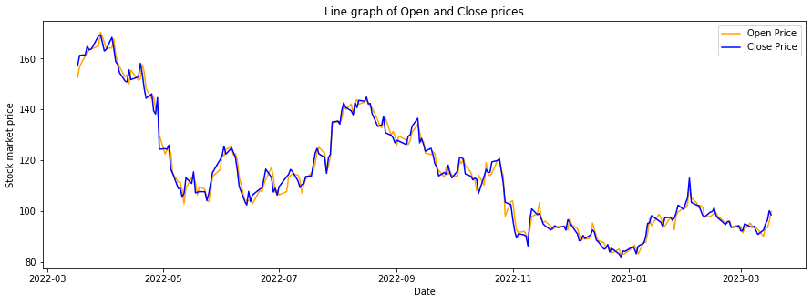
amazon[['High', 'Low']].plot(figsize = (15, 5), alpha = 0.9)

amazon[['Open', 'Close']].plot(figsize = (15, 5), alpha = 0.9)

We can infer the following patterns from the above graphs:

• Even though high and low prices differ, they don't differ by much.
• No considerable variation in opening and closing prices for a day.
• The opening price of today is very similar to the closing price of the previous day.
• The closing price is continuous except for a few days.

The above observations lead us to build a regression model using historical closing prices to predict future prices. Still, as mentioned before, the Adj closing price is a better measure compared to the closing price, so the model uses the Adj close price of the previous 15 days to predict the Adj close price for the 16th day.

Why not just take the previous 2–3 days? 
The model generally requires a good amount of data to be able to learn the pattern, and for a pattern as complex as stock prices, a time window of 2–3 days might not suffice.

Data Pre-Processing

In this step, the data needs to be transformed to remove extra feature columns and convert them into the desired format. 

data = amazon[['Adj Close']]

The data needs to be normalized, and the reason can be understood via the following example. Suppose today's closing price is $165.23 and tomorrow's is $164.12. The dollar difference will be less than $1.11, but the same in cents will be 111. To make it such that the denomination of the stock market price does not affect the model results, we should normalize it.

from sklearn.preprocessing import MinMaxScaler
scaler = MinMaxScaler(feature_range=(0,1))
scaled_data = scaler.fit_transform(data)

After pre-processing, the dataset is converted into the form of x and y, where x represents a vector consisting of the Adj closing price of the previous 15 days, and y represents the current day's Adj closing price which is the target variable.

from sklearn.model_selection import train_test_split
X_data = []
Y_data = []
for i in range(15,250):
    X_data.append(scaled_data[i-15:i,0])
    Y_data.append(scaled_data[i,0])

Finally, the converted dataset is split into three different sets; train, test, and validation.

# Let's say we want to split the data in 60:20:20 for train:valid:test dataset

# In the first step we will split the data in training and remaining dataset
X_train, X_rem, Y_train, Y_rem = train_test_split(X_data,Y_data, train_siz e=0.6)

# Splitting remaining data into 50% test data and 50% validation data
X_val, X_test, Y_val, Y_test = train_test_split(X_rem,Y_rem, test_size=0.5)

Training an ANN Model

An architecture of the ANN model is built using the Keras library of Python. The number of nodes and layers can vary and needs to be experimented with as per our prior knowledge and intuition. 

The more nodes and hidden layers the model has, the longer will be its training time. The model might also overfit if it has too many hidden layers. Here we experiment with the model having 1 hidden layer and 2 hidden layers to choose the suitable model. The below code is used for initializing a model with 1 hidden layer.

def one_hidden_layer_model():
    model = Sequential()
    model.add(Dense(10, input_shape = (x_train.shape[1],), activation='relu'))
    model.add(Dense(1, activation='linear'))

    model.compile(loss='mse', optimizer=keras.optimizers.Adam(lr=0.01), metrics=['mae', 'mse', 'mape'])
    return model

The above code has the following main components:

• Sequential() can be said to start a container where a model will be built.
• The starting layer is the input layer, followed by 1 hidden layer and 1 output layer.
• Add is used to add layers to our model container.
• Dense is the most basic type of layer where each neuron receives input from all the neurons of the previous layer.
• This being a regression problem, MSE (mean squared error) is used for calculating the loss score. 
• The number of neurons for the output layer is 1, as we only want the predicted stock market price as our output.
• The activation function used here is ReLU. We can use other activation functions like Sigmoid and Tanh to experiment with, but ReLU is the go-to choice for starting the experimentation as it fits well for many day-to-day tasks. The following image contains the graphical representations of the mentioned activation functions.

Below is a summary of the model, which has a total of 171 trainable parameters.

model.summary()
# This tells us architecture of our model
Model: "sequential_1"
_________________________________________________________________
 Layer (type)                Output Shape              Param #   
=================================================================
 dense_3 (Dense)             (None, 10)                160       
                                                                 
 dense_4 (Dense)             (None, 1)                 11        
                                                                 
=================================================================
Total params: 171
Trainable params: 171
Non-trainable params: 0

But what exactly does None in the above model summary signify?
Our model is now only initialised and not yet trained on a dataset. None represents a variable dimension of the layer, which changes as per the batch size of the input. More about batch size is discussed below.

The below code is used for building a model with 2 hidden layers.

def two_hidden_layer_model():
    model = Sequential()
    model.add(Dense(10, input_shape = (x_train.shape[1],), activation='relu'))
    model.add(Dense(10, activation='relu'))
    model.add(Dense(1, activation='linear'))

    model.compile(loss='mse', optimizer=keras.optimizers.Adam(lr=0.01), metrics=['mae', 'mse', 'mape'])
    return model

The following code is used to train the model for 1 hidden layer. Similarly, a model with 2 hidden layers can be trained.

model = one_hidden_layer_model()
model.summary()
training_logs = model.fit(x_train,y_train, epochs=100, batch_size=16, verbose=0,validation_data=(x_val,y_val))

The above code has the following main components →

• Epochs → One epoch refers to training the model with all the training data for 1 cycle. Here epochs=100 refers to repeating the process 100 times.
• Batch Size → It tells us the number of samples that will be propagated at a time through the neural network. The loss values are calculated for each batch size, which are clubbed together at the end of the epoch. For example, we have 1000 samples and a batch size of 500. Let's assume the loss values are 0.4 and 0.6 for each batch, respectively, and hence the loss value for a single epoch will be (0.6+0.4)/2 = 0.5
• Verbose → It gives us a choice to customize the expressive nature of the neural network while the model is training. Verbose=0 means nothing will be shown.
• Validation Data → This data is used to validate the neural network during the model training such that the model remains generalized and does not overfit the training data. 

After building our model, let's evaluate it on train and test datasets to get the MSE and decide on the more suitable model.

# Model with 1 hidden layer
Train loss --> 0.0014
Test loss --> 0.0010

# Model with 2 hidden layer
Train loss -->0.0015
Test loss --> 0.0011

The loss score of train and test datasets for both models is comparable, making both models suitable for our prediction purposes. 

Considering both the models are feasible, the first model is our go-to choice, as the second model is more complex and will unnecessarily increase our latency (time taken to predict and train the model). We choose the first model with a single hidden layer for predicting stock market prices.

Let's consider one more metric to show which model performs better for our use case. We consider the R-squared metric. R-squared explains to what extent one variable's variance explains the second variable's variance. It is also known as the Coefficient of Determination. 

from sklearn.metrics import r2_score
print("R_squared = ",r2_score(y_test,test_predictions))

R_squared for model with 1 hidden layer --> 0.587
R_squared for model with 2 hidden layer --> 0.515

Its values lie between 0 to 1. When closer to 1, we can say the variance of one variable affects the other's variance more. In this case, our two axis have ytest and ytest_pred, so it can be seen that the model with 1 hidden layer and an R-squared of 0.59 is a better fit compared to the 0.52 R-squared value for the model with 2 hidden layers.

But have you ever wondered how to choose the best number of epochs for the model?

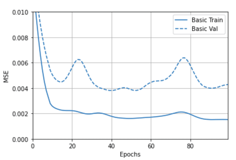
Let's decide visually by plotting a mse loss vs epoch for the model. In the plot below, after about 35 epochs, it can be seen that the loss curve for the training dataset becomes almost consistent with increasing epochs. This makes 35 the ideal number of epochs to strike a balance between loss and train time.

Performance Evaluation

After model training, let's evaluate our model using numbers and visualise the performance through graphs. After all, who doesn't want to look at the results of their hard work!!

Below are the plots of the predicted and actual values for both the test and train datasets. The more accurate our predictions are, the closer the points are situated to the y=x line. It is also evident from the higher concentration of points on the y=x line for both test and train datasets that the model is able to generalise well.

The above graph compares normalized predictions with the normalized actual values. Shouldn't the difference in actual values be much greater? 

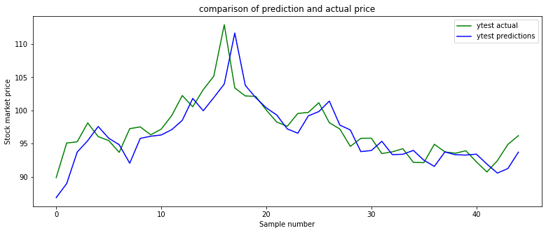
We draw a line graph to compare the actual test prices with the predicted test prices. It is inferred from the graph below that the predicted prices are closer to the actual price and on the lower side in many cases.

The above beautiful plot can be generated using the code given below.

Y_PREDICT = model.predict(x_test)
pred = scaler.inverse_transform(Y_PREDICT)
actual = scaler.inverse_transform(y_test)
plt.plot(actual , color = 'green',label="ytest actual")
plt.plot(pred , color = 'blue',label="ytest predictions")
plt.xlabel('Sample number')
plt.ylabel('Stock market price')
plt.title("comparison of prediction and actual price")
plt.legend(loc="upper right")
plt.show()

Having some numeric data to back the visual inference never hurts. We might have generally heard of accuracy as the go-to evaluation metric. Still, it cannot be used as an evaluation parameter for our use case as this is a regression model. Hence MAPE is used, which stands for mean absolute percentage error. More about it can be found in this blog.

from sklearn.metrics import mean_absolute_percentage_error
print("MAPE=" , mean_absolute_percentage_error(actual,pred))

We get a MAPE of 0.025 for our dataset, which is pretty good.

Let's compare the performance of ANN with another famous machine-learning algorithm suitable for this problem. 

Comparison of ANN and SVM

SVM, also known as a support vector machine, is an algorithm developed in the 1990s. It is widely used for regression, classification and outlier detection in the world of machine learning.

More details about SVM can be found in this blog. Here SVM is used for regression.

from sklearn import svm
regr = svm.SVR()
regr.fit(x_train, y_train)
Y_predict_svm = regr.predict(x_test)
import pandas as pd
df1 = pd.DataFrame()
Y_predict_svm
df1['pred']=Y_predict_svm
pred_svm = scaler.inverse_transform(df1)
print("MAPE=" , mean_absolute_percentage_error(actual,pred_svm))

The MAPE value for SVM is 0.029, which is higher than ANN. This shows that ANN is more effective than SVM for stock prediction. But as both are less than 5%, they are highly effective.

We now have an understanding of building a model. In the next section, let's discuss real-life scenarios related to stock market predictions.

Real-Life Fun Facts About Stock Market

1. Our model gives results very similar to the actual Adj closing price, but it is not practical to use in real life because the Adj closing price depends on many real-life features instead of just the previous prices. A straightforward example would be when Google gave a live presentation for their BARD model, but due to their negligence, an error occurred, leading to a 10% reduction in the stock prices of Google. Now, this is a real-life factor which depends on company performance.
2. Hedge Funds mainly deal in stock trading to earn their living. They don't use visualization models generally as it is slow due to the graphs involved, and even a microseconds delay can make them earn losses. So they use statistical models which are fast and help them save as much time as possible.
3. Even microseconds of getting stock market data faster for hedge fund companies are enough for them to earn profits. So they ensure that their offices are as near as possible to the stock market exchange to receive and send trading data as soon as possible.

Possible Interview Questions

• Why did you use ANN here?
• Is it a supervised or unsupervised algorithm?
• What can be done to improve accuracy?
• What algorithms can be used apart from ANN?

Related Works

• Neural Networks for stock price prediction
• Neural Smithing: Supervised Learning in Feedforward Artificial Neural Networks

Conclusion

Stock market trading is a daily occurrence on a large scale. Many stock broker platforms provide guidance to their clients on the future course of action. Large financial firms predict future prices to earn profits. All these need stock market predictions with high accuracy to work seamlessly. In this blog, we have learned to build a simple ANN model and analyze the dataset publicly available. We also discussed some real-life scenarios of stock market predictions and what factors can affect stock market predictions in real life.

If you have any queries/doubts/feedback, please write us at contact@enjoyalgorithms.com. Enjoy machine learning!