How Uber uses Machine Learning to Facilitate Surge Price?

Machine Learning and Artificial Intelligence transform the world using their applicability in many domains. More and more tech companies are leveraging such futuristic technologies to provide enhanced customer service. Uber is one such tech giant that continuously explores methods and dedicated experiments to better customer experience. It keeps on optimizing the operations and services by deploying Machine Learning-based solutions.

While using these services, we might have observed that the cab fare varies a lot for the same start and destination locations. Uber and Lyft's ride prices are not constant like public transport and are greatly affected by the demand and supply of rides at a given time. Sometimes, adverse weather conditions like rain/snow cause more people to take cab rides, affecting the service's pricing. To calculate this variation in the fares, Uber uses a state-of-the-art Machine Learning-powered Surge Pricing algorithm.

In this article, we will build a similar machine learning-based model to predict the serge multiplier based on different weather conditions.

Key takeaways from this blog

In this article, we will try to focus on these things:

• What is Surge Pricing?
• Implementation steps to predict the Surge-Pricing?
• How to visualize which features are contributing to the learning?
• How to evaluate the model performance?
• How does Uber use Machine Learning to facilitate its business?
• Possible interview questions on this project.

So, let's start with our first question.

What is Surge Pricing and how does it work?

We must have noticed that sometimes Uber charges us 1.5x–2x times the usual prices. But how does it manage to calculate this multiplier X? It is all because of the Machine Learning-powered Surge Pricing algorithm. This algorithm is used to find the most reasonable prices based on that area's economy, weather, and current traffic conditions. This algorithm uses geo-location data and demand forecasting data to position drivers efficiently. It depends on regression analysis tools to determine which locations will be the busiest to activate surge pricing in that area. This can also be used to send more drivers to that location to offer more customer-oriented services, allowing more customer retention and more profit.

We are going to implement our surge multiplier using machine learning, so let's define our problem statement more technically.

Problem Statement

The surge-pricing algorithm considers many things like the economy of any area, traffic conditions, weather conditions, etc. For this article, we will predict the weather-based surge multiplier. 

Suppose the allowed multipliers can be from this set {1, 1.25, 1.5, 1.75, 2, 2.5} and based on the weather conditions, we can try to classify which weather conditions are more favorable for which multiplier. The open-source dataset is available on Kaggle and can be found here.

Implementation Steps

Step 1: Data Description

There are two data files in the dataset: 

cab_rides.csv: Consists of the details of each ride along with its corresponding price.

weather.csv: Consists of the components of weather conditions at a particular instant of time.

The images given below show the structure of the two sets of data.

import numpy as np
import pandas as pd
from sklearn.ensemble import RandomForestClassifier
from sklearn.model_selection import train_test_split
from sklearn.preprocessing import LabelEncoder
from sklearn.model_selection import train_test_split
from sklearn.metrics import precision_score, recall_score
from sklearn.metrics import accuracy_score

cab_df = pd.read_csv("cab_rides.csv",delimiter=',')
weather_df = pd.read_csv("weather.csv",delimiter=',')

The above dataset is in the raw format, and hence we need to do some preprocessing on it before feeding it into our machine learning models.

Step 2: Data Preprocessing

First, we will try basic steps which involve data cleaning like removing null values, changing the date_time to the desired format, and other data preprocessing steps.

#convert the timestamp into the desirable format

rides['date_time'] = pd.to_datetime(rides['time_stamp']/1000, unit='s')
weather['date_time'] = pd.to_datetime(weather['time_stamp'], unit='s')
rides.head()


final_dataframe = rides.join(weather,on=['merge_date'],rsuffix ='_w')

#drop the null values rows

final_dataframe=final_dataframe.dropna(axis=0)

#make different columns of day and hour to simplify the format of date 

final_dataframe['day'] = final_dataframe.date_time.dt.dayofweek
final_dataframe['hour'] = final_dataframe.date_time.dt.hour

After preprocessing, we will merge the two datasets,

#make a coloumn of merge date containing date merged with the location so that we can join the two dataframes on the basis of 'merge_date'

rides['merge_date'] = rides.source.astype(str) +" - "+ rides.date_time.dt.date.astype("str") +" - "+ rides.date_time.dt.hour.astype("str")
weather['merge_date'] = weather.location.astype(str) +" - "+ weather.date_time.dt.date.astype("str") +" - "+ weather.date_time.dt.hour.astype("str")


# change the index to merge_date column so joining the two datasets will not generate any error.

weather.index = weather['merge_date']

# we ignored surge value of more than 3 because the samples are very less for surge_multiplier>3
surge_dataframe = final_dataframe[final_dataframe.surge_multiplier < 3]

The snapshot of the final data would be:

Feature Selection

First, we need to select the important features from the dataset. For our experiment, we have selected nine features present in the dataset affecting the surge multiplication: 'distance', 'day', 'hour', 'temp', 'clouds', 'pressure', 'humidity', 'wind', 'rain'.

# feature selection--> we are selecting the most relevant features from the dataset

x = surge_dataframe[['distance','day','hour','temp','clouds', 'pressure','humidity', 'wind', 'rain']]

y=surge_dataframe['surge_multiplier']

Label Encoding and Data Splitting

If we are solving the classification problem, then we need to label the surge multipliers present in the data {1 → 0, 1.25 → 1, 1.5 → 2, 1.75 → 3, 2 → 4, 2.5 → 5}. Once that is done, we are ready to split the data into train and test sets.

le = LabelEncoder()

#ignoring multiplier of 3 as there are only 2 values in our dataset
le.fit([1,1.25,1.5,1.75,2.,2.25,2.5])
y = le.transform(y)

feature_list=list(x.columns)
x_train,x_test,y_train,y_test = train_test_split(x,y,test_size=0.3,random_state=42)

Feature Sampling

If we try to observe the surge multiplier frequency distribution, it is evident (shown in the image below) that the data is highly imbalanced. Hence we need to apply over-sampling techniques to balance out the data. Here we have used Synthetic Minority Over-sampling TEchnique (SMOTE) over sampler.

Before SMOTE

unique, counts = np.unique(y_train, return_counts=True)
print(dict(zip(unique, counts)))

{1: 844981, 1.25: 15112, 1.5: 7042, 1.75: 3380, 2: 3029, 2.5: 187}
Train Data Before SMOTE = (873731, 9) Test Data after SMOTE = (291244, 9). NOTE: We have removed label = 3 as it had very less samples.

After SMOTE

from imblearn.over_sampling import SMOTE
sm = SMOTE(random_state=42)
train_features, train_labels = sm.fit_resample(x_train, y_train)

{1: 844981, 1.25: 844981, 1.5: 844981, 1.75: 844981, 2: 844981, 2.5: 844981}
Train Data = (5069886, 9) Test Data = (291244, 9)

Step 3: Model Training

As the price between a given source and destination is almost fixed. We need to predict the desirable surge_multiplier to get a reasonable price according to the weather condition. If we notice carefully, we can solve this problem via Regressions and the classification problem approach. Think how!

In this article, we have chosen the classification approach. We have used Random Forest Classifier and consider [1, 1.25, 1.5, 1.75, 2.0, 2.5] as 6 different classes. We can also use other classifiers like SVM or even a neural network for this problem statement.

model= RandomForestClassifier(n_jobs=-1, random_state = 42,class_weight="balanced")

model.fit(x_train,y_train)
y_pred=model.predict(x_test)

Step 4: Feature Importance

It is always a good practice to see the dependency of our model on different features. An additional advantage of Random forest is that the importance of every feature comes as a by-product of training.

# Get numerical feature importances
importances = list(model.feature_importances_)
# List of tuples with variable and importance
feature_importances = [(feature, round(importance, 2)) for feature, importance in zip(feature_list, importances)]
# Sort the feature importances by most important first
feature_importances = sorted(feature_importances, key = lambda x: x[1], reverse = True)
# Print out the feature and importances 
[print('Variable: {:20} Importance: {}'.format(*pair)) for pair in feature_importances]

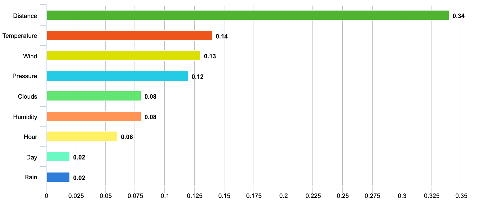
It can be seen that the model is dependent on the distance feature the most and subsequently on the other features represented in the decreasing order of importance.

Step 5: Evaluation of the built model

from sklearn.metrics import accuracy_score
from sklearn.metrics import f1_score
f1_score(test_labels, predictions, average='weighted')
accuracy_score(test_labels, predictions)

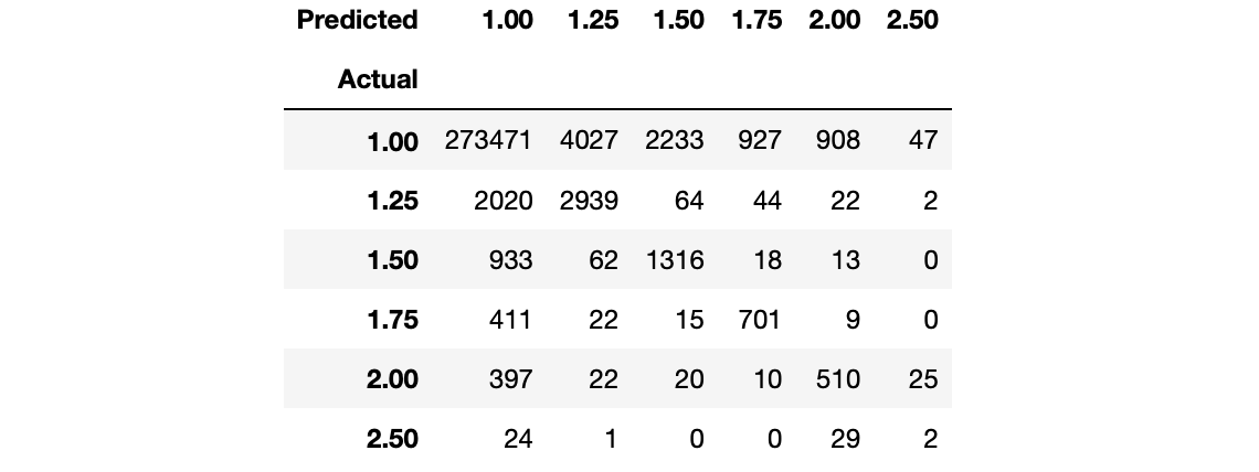
For the model we built, F1-score is 0.9616, and the Accuracy is 95.77%. So we can say that the ML model is doing quite a decent job here. The below diagram shows the complete confusion matrix.

How does Uber use Machine Learning to facilitate business?

We must be familiar with Uber and how easy it is to use its service. We only need to open the app and book a cab, the cab comes and takes us to our destination point, and we pay the driver after the ride's completion. Isn't that too simple?

In reality, it is not as simple as it appears from the outside. Behind offering such a simple user experience, Uber runs many background services and complex algorithms. The critical component which is making it possible is Machine Leaning. Let's see how Uber utilizes Machine Learning to offer seamless services for a better customer experience.

1. Adequate demand-supply chain

Uber deals with a large amount of data daily. It forecasts the location and time of the demand by exploiting both the stored and the real-time data coming from the users' app. Using these estimates, the app notifies the drivers to meet the demand requirements in a particular area. Hence in this manner, Uber manages and balances demand and supply chain and offers customer-centric services.

2. Fare Estimates

Machine Learning enabled Demand Forecasting allows Uber to play with the prices during peak hours to increase profit. Increasing the price is never an easy solution as it also comes at the cost of customer retention. Uber calculates fares using real-time traffic data. It analyses various external factors that could affect the fares, such as public transport availability and how accessible these public facilities are, etc.

3. Customer Retention

The gap in the demand-supply chain could result in the unavailability of cabs. Such circumstances may result in users booking a ride from different available services like Ola in India. Uber's machine learning-based demand predictions play a crucial role in customer retention. It uses both historical and real-time data to bridge the gap between demand and supply.

4. Accurate expected time arrival

It might be very frustrating for the users to wait for the cabs to reach a pickup location. Using Machine Learning-based approaches, Uber uses real-time traffic and GPS data and Map APIs to forecast the expected arrival time. Specific steps can be taken to decrease the expected time arrival (ETA) when customers book rides. Uber always focuses on providing a superior customer experience by reducing the user's waiting time.

5. Route Optimization

Uber uses a Machine Learning-based system to predict the best routes and recommend the most optimal ones to the drivers. Using its accurate route optimization system, it assists drivers in avoiding crowded areas. Traditionally, the route selection was based on absolute presumption and behavioral estimation of the driver. They didn't consider any real-time traffic, road blockage, and other weather conditions. Machine Learning-based systems incorporate all these parameters and offer the best services.

6. Uber Pool

Uber has introduced the Uber Pool services that allow shared riding to combat cabs' difficult unavailability during peak hours. Uber Pool allows ride-sharing between the riders heading in the same direction and will enable customers to have an economical ride at a lesser price. Uber uses Machine Learning based algorithms to identify possible matching rides and assign them the same cab. Such an advanced system also decides whom to pick first and drop first. Uber Pool also uses the stored data to find out the hidden pattern and accordingly modify the prices to offer the best services to its customers and, at the same time, manage higher profits.

7. Big Data and Uber

Uber systems collect and maintain a large amount of data, use big data processing techniques, and offer more personalized services. It solely relied on Hadoop and Spark frameworks for real-time processing of large-scale Machine Learning based algorithms. 

It maintains a massive database of drivers simultaneously, matching any ride to that particular driver in just 10–15 seconds. Uber closely observes each ride and its associated data to predict more accurate demand-supply chain prices and allocate sufficient resources according to the need. It considers various external data such as the availability of public transport facilities and many external factors.

Possible Interview Questions

Based on this project, an interviewer can ask these questions in any data science and machine learning interview:

• What are the different techniques that Uber uses to retain the customer?
• Here you have solved the classification problem. Can this be solved as a regression problem? Which algorithms will be used in the regression problem?
• What is Ensemble learning? Is Random Forest an Ensemble learning approach?
• Why don't we use the decision tree directly? Why Random Forest?
• What methods will you propose to increase the accuracy from this point?

Conclusion

The swift progress of Machine Learning tools and techniques is continuously bringing favorable circumstances to offer customer-oriented services and intensify several businesses' productivity. Uber has emerged as a big business using machine learning-based systems and focusing more on offering customer-oriented services. Artificial Intelligence and Machine Learning backed system helps offer optimized services and is also highly useful for adding and retaining customer service. In this article, we implemented one of the use-cases of Uber using the Machine Learning based approach. We hope you have enjoyed it.

Enjoy Learning, Enjoy Algorithms!