Introduction to Artificial Neural Networks

All types of Machine learning models can be classified into three categories based on the nature of the algorithm used to build that model. These are Statistical Machine Learning, Artificial Neural Networks, and Deep Learning. Traditional Machine Learning approaches failed to learn complex non-linear relationships in the data, and ML engineers wanted an approach to tackle these challenges.

That's when Artificial Neural Networks (ANNs), also called Neural Networks, got discovered after deriving inspiration from the human brain. While the comparison between ANNs and the human brain is superficial, it helps us understand ANNs more simply. It is a supervised learning algorithm capable of solving classification and regression tasks. This article will set a foundation to dive deeper into this field.

Key takeaways from this blog

After going through this blog, we will be able to understand the following things:

• An analogy from the human brain to understand how neural networks work.
• Explanations of the terms constituting the definition of neural networks
• Key insights from the schematic diagram of neural networks.
• Advantages and disadvantages of neural networks.
• Practical use-cases of neural networks in real life.

Let's start the journey toward diving deeper into the domain of Machine Learning.

An analogy from the human brain to understand Neural Networks

The human brain is a complex system, and its working is still a mystery in medical science. It learns and adapts through the self or others' past experiences. Neurons, the brain's basic building blocks, play a crucial role in this process. Billions of such neurons form connections inside our brains and store the learned experiences as memories. When our sensory organs, such as our eyes, skin, and ears, encounter similar situations, the brain uses those memories and responds similarly.

An example of this is learning to drive a car. Our brains experience various situations on the road and learn how to respond. Once learned, the brain uses signals from our eyes, nose, and ears to control the vehicle's various parts. When we encounter new situations, the brain adapts and modifies the stored learnings. We can correlate this scenario to learning a mapping function on input and output signals and give responses whenever similar information comes. 

This process is mimicked in neural networks, where these algorithms use interconnected neurons to map the complex non-linear functions on the input and output data.

Formal Definition of an Artificial Neural Network

If we define neural networks in plain English, we can say: 

“Artificial Neural Networks are user-defined nested mathematical functions with user-induced variables that can be modified in a systematic trial-and-error basis to arrive at the closest mathematical relationship between given pair of input and output.”

Let's know each of the terms used in the above definition, and then we will define it in our terms.

User-defined

In any field of machine learning, machines try to map mathematical functions on input and output pairs. But there can be infinite possibilities to search on which function would be best-fit on input and output sets. Our ML algorithm may take forever to find the perfect function. Hence, it raises the question of how machines decide this should be the mapped function. 

Machines need help here. We need to provide some starting point to machines by defining a mathematical function that includes adjustable parameters. With this, the machine's search becomes limited, allowing for more efficient and effective learning.

To understand this better, correlate the scenario with what we did while developing the Linear Regression model. We need to precisely define that this degree of polynomial should be fitted on the given dataset. For example, for fitting a three-degree polynomial, we started with this function: Y_predicted = θ3* X³ + θ2* X² + θ1* X + θ0. Machines try to find the optimal values of θs. 

User-induced variables 

These are the θs in the above equation. ML models attempt to find the optimal values for the parameters that make the final function as similar as possible to the actual function. But what's the benefit of tuning the parameters?

Neural networks are supervised learning algorithms, meaning the algorithm will have information about the true output while training. By tuning the parameters, ML algorithms will ensure that their predictions should be as close as possible to the true values. 

These parameters, also known as weights, assign importance (weightage) to the input parameters. For example, in the function Output = 2*Input + 3, the value 2 represents the weight applied to the input. If the input has multiple features, machines will set the importance for each feature. In simple terms, if the input vector is multi-dimensional, the weight vector will also be multi-dimensional. 

These weights are trainable parameters and are modified based on the input and output samples during the learning process.

Mathematical Functions

Machine Learning models represent the relationship between input and output pairs as mathematical functions. These functions have two main components:

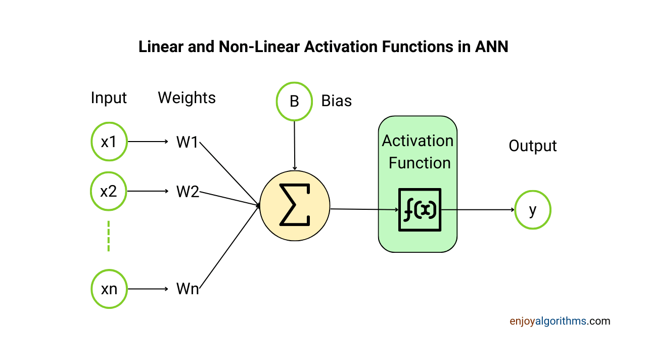
1. Aggregation Function: The inputs to the defined mathematical function are modified by multiplying weights and then adding biases. These weights and biases are nothing but user-induced variables. This process is similar to what we did in Linear Regression, and that's why this step is also known as the Linear step in Neural Networks.
2. Activation Function: Neural networks were introduced to extract complex non-linear relationships hidden in data. Activation functions are applied to the weighted output of the aggregated function (Linear step) to introduce non-linearity in the input-output relationship. This nested non-linearity allows the model to learn complex patterns present in the dataset. In later posts, we will delve deeper into the various types of activation functions and their uses.

Nested mathematical functions

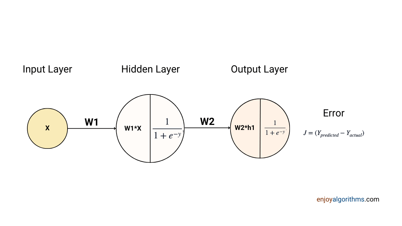
In the diagram below, there is a single neuron in the hidden layer, but in practice, there can be multiple neurons in one or multiple hidden layers between the input and output layers. Schematically, the input of the first hidden layer is the input layer, and the output of the first hidden layer serves as the input for the second hidden layer. The final output from the output layer is the desired output from the neural network.

So, if a function exists between the Input layer and the first hidden layer, the output for this function will be used as input to the function present between the first and second hidden layer, and so on. When we look at the overall process in Neural Network, it will seem like a complex composite function, which is nothing but a nested mathematical function: f1(f2(…fn(x))..).

Trial-and-error basis 

The error function measures the difference between the ML model's predicted and true values. When we average this error over all the data samples, it becomes the cost function. The goal of the ML algorithm is to minimize this cost function by adjusting the values of user-induced variables. 

In neural networks, this cost function can have multiple minimum values. Out of all these minimum values, we want to reach the position of global minimum of the cost function. Hence, adjusting the parameters gradually ensures that the cost function reaches a global minimum.

Systematic: 

If the user-defined mathematical function cannot capture the complex patterns in the data, a different form of the mathematical function may be used, or the algorithm's complexity can be increased. This process of adjusting the function is done systematically to ensure that the model should learn what is required from the data. 

Closest mathematical relation

One question must be coming to our mind, Why do machines not learn the exact values for the parameters so that they predict exactly equal to the true values?

Our objective in machine learning is to give predictions as close as possible to the actual values. But, Sometimes, with the constraints of computing power and time limit, we settle with the closest function rather than trying continuously to make error zero. 

For example, a user-defined mathematical function may be aX + b, where X is the input variable and [a and b] are user-induced variables that the machine can adjust while finding the best mathematical relationship. However, suppose the actual dataset follows the mathematical function 2X + 3. In that case, the machine may only be able to find a mathematical relationship close to the actual one, such as 1.9X + 3.2, based on the given samples and the number of iterations it was allowed to perform. This result is not an exact match, but it is the closest approximation the machine could find based on the given conditions.

Comparing ANNs with Directed Acyclic Graph

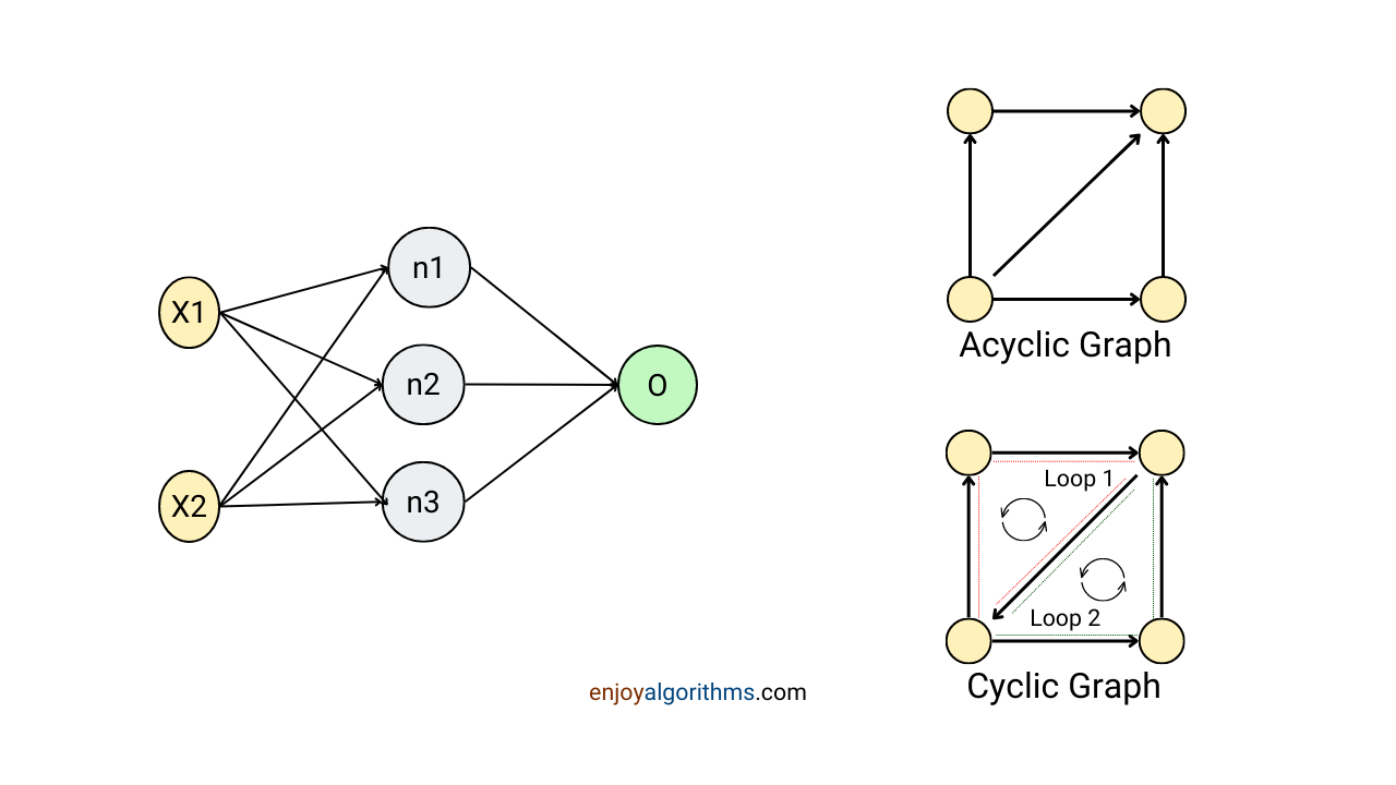
Graphs are very popular in Data Structures and Algorithms. If we observe the Neural Networks closely, it is nothing but a particular type of graph where every node is directed towards another node in an acyclic manner. In DSA, this type of graph is popularly known as DAG (Directed Acyclic Graph). When we define Neural Networks in our programs, we need to define each node of the graph to form a directed acyclic graph. 

A directed graph is where every connection between the nodes (vertices) is directed from one node to another. If one follows this direction, one will not revisit the same node. This property is also quite prevalent in Neural Networks, as data samples move from the input layer toward the output layer. 

---

What information is needed to design an Artificial Neural network?

With all the above information, we might have understood what exactly is present in any Neural Network. Now let's learn how exactly this nestedness work.

When designing the structure of Neural Networks, it is crucial to consider the following:

• Each neuron in the input layer corresponds to one input feature of the dataset. So if the dataset has 50 input features, the Input layer will have 50 neurons.
• The number of output categories determines the total number of neurons in the Output layer. For example, if there are 10 categories in the output, the Output layer will have 10 neurons. If we use ANNs for regression problems, one node in the output layer will predict the continuous label. 
• The number of hidden layers and the Number of Neurons in each hidden layer are pre-defined in the network and are not trainable parameters. These non-trainable parameters are called hyperparameters and are tuned based on multiple experiments on the same dataset. Although some heuristics help guess these values, we will learn this in a separate blog.
• Every neuron in any layer is connected to every neuron in the adjacent layers. For example, if hidden layer 1 has 20 neurons and hidden layer 2 has 60 neurons, every 20 neurons in hidden layer 1 will be connected to all 50 neurons of the input layer and all 60 neurons in hidden layer 2. Sometimes these connections need to be dropped as the model starts overfitting the dataset. We will learn more about this in the drop-out regularization technique. 
• In every neuron, either from the hidden layer or the output layer, there exists one trainable parameter called bias, and every connection between neurons is weighted by a trainable variable called weights. These weights and biases are collectively called the weight matrix.
• We need to define the activation function for all the hidden and output layers to introduce non-linearity in learning. We have covered the basics of the Activation function in a separate blog.
• In a Neural Network with 50 features in the input, 10 output categories, 20 neurons in hidden layer 1, and 60 neurons in hidden layer 2, the total number of trainable parameters will be:
  Biases (for every neuron from the hidden and output layers) = 20 + 60 + 10 = 90, and Weights (for every connection between neurons) = 50*20 + 20*60 + 60*10 = 2800, so the total trainable parameters will be 2890. As the number of parameters increases, the ANN model becomes complex and computationally expensive.
• Apart from architectural things, some common principles will be followed as we did in Machine Learning. We need to define the cost function to train the Neural Network and use optimation algorithms to reach the global minimum of the cost function. These topics will be covered in separate blogs.

Advantages of Neural Networks

Some of the key benefits of using Neural Networks are:

• Neural Networks can learn complex non-linear relationships between input and output data, making them well-suited for complex classification and regression problems. For example, Image Classification, Essay Grading, and Bounding box prediction.  
• They can generalize their learning to new, unseen data and make predictions with a high degree of accuracy.
• In traditional ML algorithms, we demand homogeneous distribution in the dataset. For example, all the data samples should come from the Gaussian distribution to get better performance from the Linear Regression model. But, the distribution of the input data does not limit Neural Networks and can work well with data that follows heterogeneous distributions. This makes them versatile and suitable for a wide range of data types.
• Neural Networks are robust to noise/outliers present in the data, meaning their predictions are not significantly affected by random variations in the dataset.

Disadvantages of Neural Networks

While Neural Networks have many advantages, there are also some drawbacks. Some of them are:

• Training Neural Networks can be computationally intensive and require powerful hardware. As the number of hidden layers or nodes in the hidden layer increases, the need for higher processing power also increases.
• One of the main disadvantages of Neural Networks is their lack of interpretability. They cannot explain how or why they arrived at a certain prediction, sometimes making it difficult to understand and trust their results. 
• There is no fixed method for designing Neural Networks, and the design includes hyperparameters such as the number of layers, the number of neurons, and the type of activation functions. All these hyperparameters must be fine-tuned through multiple experiments.

Practical use-cases of Neural Networks in real life

Neural Networks are particularly well suited for those problem statements where the datasets exhibit high levels of non-linearity. For example:

• Optical Character Recognition (OCR): OCR is a complex problem that involves highly complex non-linear relationships between the characters in an image. Neural Networks can process a large amount of input, such as a complete image represented in matrix form, and automatically identify which characters are present. This makes them well-suited for OCR, facial recognition, and handwriting verification applications.
• Stock market price prediction: Forecasting stock prices is challenging, as market behavior is often unpredictable. However, many companies now use Neural Networks to anticipate whether prices will rise or fall in the future. By making more accurate predictions based on past prices, Neural Networks can help companies make significant financial gains.

Conclusion

Artificial Neural Networks is a supervised learning algorithm that solves classification and regression problems. This is considered a fundamental concept in Deep Learning, and we learned the basics in this article. We learned about the information required to design an ANN and its advantages and disadvantages. In upcoming blogs, we will dive deeper into the components of ANN. 

Enjoy Learning!