Dynamic Programming in Data Structures and Algorithms

Divide and conquer approach helps us to design efficient solutions when subproblems are independent. When sub-problems are dependent or repeated, divide and conquer strategy does much more computation than expected, which leads to an exponential time solution. Such types of problems can be efficiently solved using a dynamic programming approach.

In dynamic programming, we also solve problem by combining solutions to subproblems. But rather than solving same sub-problem repeatedly, we solve each sub-problem once and store calculated value in extra memory or look up table to avoid recomputation. When same sub-problem appears again, we return already stored solution in the memory. This is an idea of Time-Memory Trade-Off, where we use extra space to improve time complexity from exponential to polynomial time.

From a coding interview and application perspective, dynamic programming is one of the most popular problem-solving techniques to master. Before moving forward to idea and implementation steps of dynamic programming, let’s start by understanding a critical challenge with the recursive solution of finding nth Fibonacci.

Recursive solution of finding nth Fibonacci 

In the Fibonacci sequence, every number is the sum of two preceding numbers. For example: 0, 1, 1, 2, 3, 5, 8, 13, 21, 34, 55, 89, 144, …. So we can easily define recurrence relation to calculate nth terms of Fibonacci using (n - 1)th and (n - 2)th term.

Recursive structure: fib(n) = fib(n - 1) + fib(n - 2) 
Base case: fib(0) = 0 and fib(1) = 1

Here we are solving the problem of finding nth Fibonacci using the solution of finding (n — 1)th and (n — 2)th Fibonacci, where fib(0) and fib(1) are base cases. So we can easily implement the recursive solution by combining the solution of these two sub-problems.

Pseudocode of finding nth Fibonacci using recursion

int fib(int n)
{
    if (n <= 1)
        return n
    else
        return fib(n - 1) + fib(n - 2)
}

Time complexity analysis of recursive nth Fibonacci

The above solution looks simple and elegant, but it is highly inefficient. Let’s understand the reason by creating recursion tree diagram.

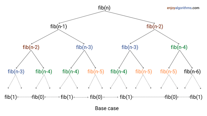
There are two recursive calls and one addition operation at each step of recursion. In other words, we are doing O(1) operation at each recursive call. So time complexity of finding nth Fibonacci = O(1) * (Total number of recursive calls)

The recursive calls are growing exponentially level by level i.e. 1, 2, 4, 8, 16…, and so on. If we assume that the above tree is full at each level, then the height of recursion tree = n. So total number of recursive calls = 1 + 2 + 4 + 8 …+ 2^n = 2^(n +1) — 1 = O(2^n) [Using the summation formula of geometric series]. So time complexity = O(2^n) * O(1) = O(2^n). 

Critical observation: Input size decreases by 1 on the left side and by 2 on the right sides. It means: The height of the leftmost leaf node will be n and height of rightmost leaf node will be n/2. So the height of leaf nodes will be in the range of [n/2, n]. What would be the precise analysis? The answer is approx equal to (1.6)^n, which comes from the properties of Fibonacci series. Explore and think!

Overall, recursive algorithm of finding nth Fibonacci is a highly inefficient algorithm. Even it will take a long time to generate output for small values of n like 30 or 50 or 70. The critical question is: Why time complexity is growing exponentially? The idea is simple: We are solving same sub-problems again and again during recursion. For example, fib(n - 2) is calculated 2 times, fib(n - 3) is calculated 3 times, and so on. If we move down the recursion tree, the count of repeated sub-problems will increase.

So, due to repeated calculation of sub-problems, time complexity is in exponential order of n. The critical question is: Can we stop repeated computation and improve time complexity? Yes, here comes the awesome idea of dynamic programming! There are two popular techniques to solve problem using dynamic programming: 1) Top-down approach (Memoization) 2) Bottom-up approach (Tabulation)

Top-down approach (Memoization)

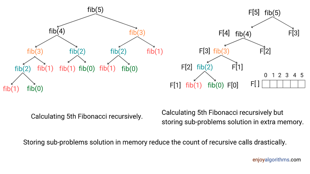
Top down approach of dynamic programming is an just an optimized version of the inefficient recursive approach. Here, instead of solving same sub-problems several times, we store their solutions in an extra memory when we encounter the sub-problem first time during recursion. If we again encounter the same sub-problem during recursion, we first check for their solution stored in extra memory. If sub-problem solution is already calculated, we return that value instead of calculating that sub-problem again.

There is a critical question: What would be the size of extra memory? The idea is simple: We need to allocate extra space to store solution of every unique sub-problems encountered during recursion. In other words, the size of extra memory is equal to total number of different subproblems. One more important thing: We need to initialize the table with some empty flag or value to identify that sub-problem solution is not calculated yet.

Let’s understand this using the example of finding nth Fibonacci problem.

Fibonacci solution using top-down memoization 

There are total n + 1 different sub-problems in the recursive solution of finding nth Fibonacci, i.e. fib(0), fib(1), fib(2)….., fib(n-2), fib(n-1) and fib(n). So we need extra memory of size n + 1 to store the solution of different sub-problems. Let’s say F[n + 1].

Now we initialize all values in the table with -1, as the value of Fibonacci can’t be negative. This will help us to check whether the solution of sub-problem has already been computed or not. Now we are ready to modify the recursive solution.

• If(F[i] < 0): The value of ith Fibonacci has not been computed yet. So we calculate the solution recursively and store it at ith index i.e. F[i] = fib(i — 1) + fib(i — 2). Note: Initial value of i will be n.
• If (F[i] > 0): The solution of ith Fibonacci has already been calculated and stored at F[i]. So we don’t calculate it again and return the value stored at F[i].
• By the end of above process, solution to the sub-problems will be stored in the table. So as a final solution, we return value stored at F[n].

The role of base case is critical in this process, and we need to define it correctly (Think!). A base case is a situation when recursion reaches the scenario of n = 0 and n =1, for which we already know the solution. So, we can directly store 0 at F[0] and 1 at F[1].

Pseudocode of nth Fibonacci using the top-down approach

Initaize F[n + 1] with -1.
int fib(int n)
{
    if (n <= 1)
        F[n] = n
    else if (F[n] < 0)
        F[n] = fib(n - 1) + fib(n - 2)
    else
        return F[n]
}

Time and space complexity analysis

At each stage of recursion, there are two sub-problems, and we solve each sub-problem only once. The total number of recursive calls = n + n — 1 = 2n — 1 (We are solving n + 1 sub-problems only once). So time complexity = O(n). Space complexity = O(n) for n + 1 size extra array to store the solution of subproblems.

An intuition of bottom-up approach from top-down approach

In the top-down approach, if we observe the flow of recursive calls to store results in the table, we can get insights related to bottom-up approach of dynamic programming. How? Let’s think!

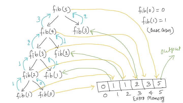
When we call fib(n), recursion will come top-down, calling the larger problem (Input size n) to the smallest version of the problem (Input size 0 and 1). So it will first store value at F[0] and F[1]. In other words, it will keep storing values from smaller problems to larger ones, where F[0] and F[1] are the first two values stored in the table.

Order of execution of recursive calls: 

fib(n)-> fib(n-1)-> fib(n-2) …-> fib(i)-> fib(i-1)-> fib(i-2)…-> fib(2)-> fib(1)-> fib(0)

Order of storing the results in the table

F[0]-> F[1]-> F[2] …-> F[i]-> F[i-1]-> F[i-2]…-> F[n-2]-> F[n-1] ->F[n]

So one idea is simple: Rather than using top-down approach, we can store results incrementally in a bottom-up fashion. In other words, we can start by storing the solution for input sizes 0 and 1 and move forward to store the solution for the larger sub-problem iteratively. Think!

The bottom-up approach to dynamic programming

This is the most popular way to solve dynamic programming problems. As seen in the above section, we can solve smaller problems first and then combine their results to build the solution to a larger sub-problem. We can implement this using simple loop for storing results in a table.

Let’s understand and visualize this approach using the example of finding the solution of nth Fibonacci.

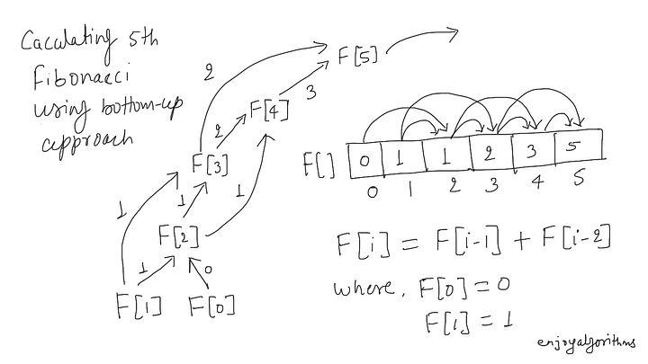
Fibonacci solution using the bottom-up approach

Step 1: Defining Table Structure

To store the solution in a bottom-up approach, we first need to define the table structure and size. Here, we have only one variable on which the state of problem depends, which is n (The value of n decreases after every recursive call). So, we need to define an one-dimensional array to store sub-problems solution.

Step 2: Defining Table Size

The total number of different subproblems defines the size of this table. If we observe the recursion tree, there can be total (n + 1) different sub-problems.

Step 3: Table Initialization

We can initialize the table by using base cases. This could help us to fill the table and build solution for the larger sub-problem. F[0] = 0 and F[1] = 1.

Step 4: Defining Iterative Structure to fill the Table

We should define an iterative structure to fill table by using the recursive structure.

Recursive structure: fib(n) = fib(n-1) + fib(n-2)
Iterative structure: F[i] = F[i-1] + F[i-2]

Step 4: Termination and returning the final solution

After storing solutions in a bottom-up manner, our final solution gets stored at the last Index of the extra array i.e. return F[n].

Pseudocode of nth Fibonacci using bottom-up approach

int fib(int n)
{
    int F[n + 1] 
    F[0] = 0
    F[1] = 1
    for (int i = 2; i <= n; i = i + 1)
        F[i] = F[i-1] + F[i-2]
    return F[n]
}

Time and space complexity analysis

We are using a table of size n + 1 and running single loop to fill the table. Time complexity = O(n), Space complexity = O(n).

Subproblem graphs in dynamic programming

In a dynamic-programming problem, we must identify subproblems and their dependency on each other. To understand this idea, let’s understand the concept of subproblem graph.

The sub-problem graph is a directed graph of sub-problems, where we have one node for each unique sub-problem. It has a directed edge from the node of subproblem p to subproblem q if solution of subproblem p involves solution of subproblem q.

For example, bottom-up approach considers nodes of a subproblem graph in such an order that we solve the subproblems q adjacent to a given subproblem p before we solve subproblem p. This will create nodes of the subproblem graph in reverse topological order of sub-problems. Think! In other words, no subproblem is considered until all of the subproblems it depends upon have been solved.

The size of the subproblem graph can help us determine the dependency and order in which we need to build solutions in a bottom-up manner. On another side, the time to compute the solution to a subproblem is proportional to the degree (number of outgoing edges) of the corresponding vertex in the subproblem graph, and the number of subproblems is equal to the number of vertices in the sub-problem graph. In this common case, the running time of dynamic programming is linear in the number of vertices and edges.

Why is DP popular during coding interviews?

Dynamic programming is important during coding interviews due to several reasons:

• There is a lot of variation available to dynamic programming problems.
• There can be a possibility to optimize the time and space complexity of dynamic programming solutions. Sometimes we can optimize DP solution from O(n²) to O(n) time or O(n²) space to O(n) or O(1) space.
• It is one of the best ideas to evaluate the understanding of problem-solving using iteration and recursion.

Real-life application of dynamic programming

• Sequence alignment, Document diffing algorithms, Document distance algorithm (Edit Distance), Plagiarism detection, Typesetting system
• Duckworth Lewis Method in cricket, Flight control
• Speech recognition, Image processing, Machine learning algorithms
• Economics, Financial Trading, Bioinformatics, Operations research

Critical ideas to explore further

• How do we recognise a DP problem?
• Top-down vs bottom-up approach
• Dynamic Programming vs Divide and Conquer
• Dynamic Programming vs Greedy Approach
• Patterns of problem-solving in dynamic programming

Suggested problems to solve

• Longest common subsequence
• Maximum subarray sum
• Climbing stairs problem
• Minimum number of jumps to reach the end
• Minimum coin change problem

References

• Algorithms by CLRS
• Algorithm Design Manual by Skiena

Happy coding. Enjoy algorithms.