Music Recommendation System Using Unsupervised Learning

In the current world, music apps like Gaana and Spotify are competing with each other to increase their recurring users. We might think, if both are song apps, then how does it matter which app we should use? An app that provides a better UI interface, a lesser latency, i.e., time taken to load the app, better music recommendations, lesser cost of subscription, and more available songs for users attracts more customers. In all the above points, Machine learning is closely involved in music recommendation. 

Music recommendation predicts songs users might like to hear based on their previous listening history. A better recommendation system is considered one of the key technologies responsible for the success of Netflix and Amazon PrimeVideo. In this blog, we will develop recommendations for songs that can help businesses significantly increase recurring users on their platforms.

Key takeaways from this blog

• Different Methods to build a recommendation system for songs
• What are various Audio Features available?
• Step-wise Implementation of music recommendation system
• Ordering Songs for Recommendation
• Brain think tank

Let us learn about different types of recommendation systems. Our next section will discuss the advantages of using audio features over the traditional approach.

Different Methods to build a recommendation system for songs

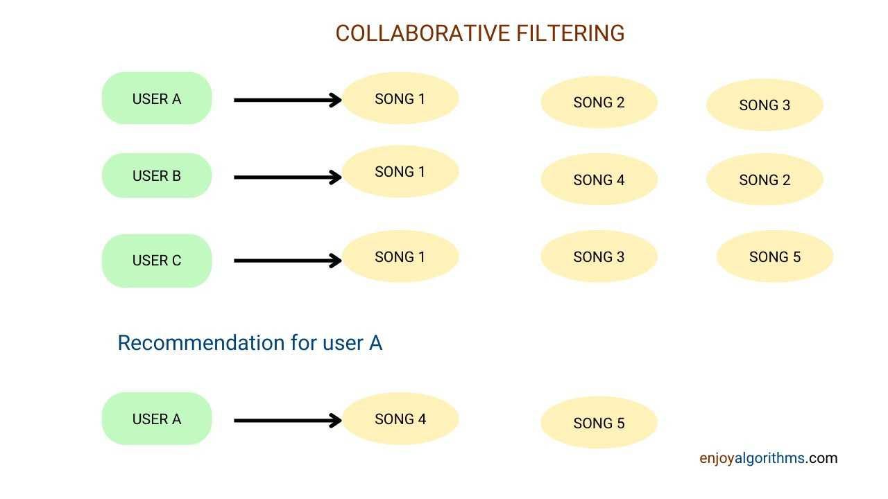
• Collaborative filtering → This refers to giving recommendations to users based on others who might have a similar listening pattern. Here we use algorithms like word2vec, ALS, etc.

• Using Features of music → Here, we do not have any relation to user listening history, and we recommend songs based on the similarity in music features. These features can be of two types:
  1. Meta Data → This includes features like release year, duration of the track, artists, album, music tags, and composer, i.e., which tell us more about the song but are not related to audio.
  2. Audio Features → These include features related to audio like tempo, pitch, loudness, etc.

In today's world, collaborative filtering is one of the industry's most used methods for building recommendation systems. But this system shortfalls in the discovery aspect. We only recommend songs to users listened to by a group of users. This often leads us to a self-serving loop where users listen to the same tracks and miss out on the discovery aspect. This issue can be solved using audio features that describe the essence of songs for us.

Here in this blog, we see how to use audio features to build a recommendation system. So let's learn about these audio features in greater detail.

What are different Audio Features available?

We extract audio features in Audio signal processing (a subfield of signal processing). AFP(Audio features in reference to blog) or audio fingerprints refers to extracting audio features in numerical numbers such that we can identify unique sounds. In Python, we can use libraries like essentia and librosa to extract such audio features. Some of the primary audio features are:

• Loudness → Steven's power law helps calculate loudness, defined as signal energy to the power 0.67.
• Tempo → It is defined as beats per minute, also known as BPM.
• Pitch → Fundamental frequency of any audio waveform
• Energy → Root mean square of signal magnitude
• Zero Crossing Rate → The number of times the audio waveform crosses the zero axis.
• Chroma → These features represent the 12-length vector which gives us numerical values corresponding to 12 distinct semitones of music.
• MFCC → It stands for Mel-frequency Cepstral coefficients. This feature MFCC is understood to represent the filter (vocal tract). In simple terms, we can use it as a filter for the singers.

Some engineered features from audio are:

• Danceability → Here, we rate the danceability of a song on a scale of 0–1. It tells us how likely the song can be a dance song and is based on various features like pitch, loudness, tempo, etc.
• Chorus → It tells us about parts of songs that are repeated continuously, like a line repeated in a song.

We had enough of theory. Now let us jump into its Implementation. Please note that there is no labeled data here, so it will be an unsupervised problem. We will be using the famous k-mean algorithm. 

Steps to Implement Music Recommendation System Using Audio Features

Step 1: Dataset description for Music Recommendation System

We will use Million Song Dataset. The complete dataset is a 300GB dataset where we can find all the metadata and audio features of different tracks. As this is a huge dataset, we will take a subpart of the dataset for roughly 2000 songs. All features are present in h5 format, which stands for hierarchical data format 5. Every single file can approximately have data for a single song. We can access the h5 format using pytables in Python. 

import hdf5_getters
h5 = hdf5_getters.open_h5_file_read(path to some file)
duration = hdf5_getters.get_duration(h5)
h5.close()

We have dropped meta-features for our blog, focusing on audio features. Also, we have features like segment_timbre (basically MFCC and has shape (segment length, 12)), where a song is divided into several segments, and features are available for each segment. 

If we extract more features, the model's accuracy will increase, but the time complexity will also increase. So to solve this tradeoff, we have taken an average over the whole song instead of having features for each segment. So segment_timbre for each segment became MFCC1, MFCC2, MFCC3 … MFCC12 for the entire song (shape changes to 1*12). We have stored this modified dataset in a CSV format. Let's see the top 5 rows of our new dataset.

import pandas as pd
df = pd.read_csv('million_song_subset.csv',sep='###')
pd.options.display.max_columns = 10
df.head()

df.columns
##Names of all columns in dataset we get
Index(['song_id', 'song_title', 'duration', 'year', 'danceability', 'energy','loudness', 'tempo', 'time_signature', 'segment_loudness_avg','chroma1', 'chroma2', 'chroma3', 'chroma4', 'chroma5', 'chroma6', 'chroma7', 'chroma8', 'chroma9', 'chroma10', 'chroma11', 'chroma12','MFCC1', 'MFCC2', 'MFCC3', 'MFCC4', 'MFCC5', 'MFCC6', 'MFCC7', 'MFCC8''MFCC9', 'MFCC10', 'MFCC11', 'MFCC12'],
  dtype='object')

Please note that apart from audio features, we have some extra columns, like:

• song_id → It helps us identify unique songs
• song_title → It tells us the name of the songs
• duration → It tells us the length of songs in seconds
• year → It tells us the release year of the song

Here we also have an audio feature that was not discussed earlier: time_signature → time signature of the song according to The Echo Nest, i.e., the usual number of beats per bar.

We analyzed the columns in our dataset and found that some features do not add much value to model development. For this purpose, we used multiple visualization techniques. Let's see some of those data visualizations in the next section.

Step 2: Data Visualization for Million Song Dataset

Let's see the histogram plot first.

import matplotlib.pyplot as plt
df.hist(figsize=(15,15))
plt.tight_layout()
plt.show()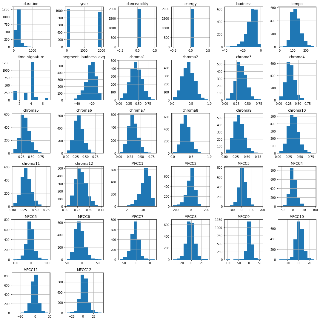

The above plot shows that chroma1 is uniformly spread between 0 and 0.75, while features like year and duration mainly have two values. There is also danceability and energy, which only have single values. This might look strange as the value remains the same for all 2000 songs. So we drop features like duration, year, danceability, and energy as they do not change much for all 2000 songs and will not provide new insights for our model.

df1 = df.drop(['duration','year','energy','danceability'] , axis=1)

Let's draw a heatmap to see the relation of features with each other.

import seaborn as sns
plt.gcf().set_size_inches(15, 15)
cmap=sns.diverging_palette(500,10,as_cmap=True)
sns.heatmap(df1.corr(),center=0,annot=False,square=True)
plt.show()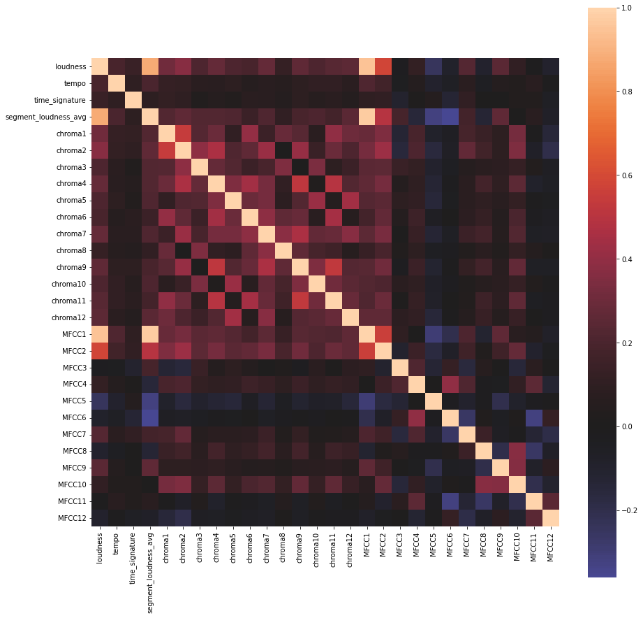

All features are linearly related to themselves, which is expected by logic. We have many dark black places corresponding to zero, which shows that these features are independent and do not affect each other.

Now that we have analyzed the data let's preprocess before feeding it into the model.

Step 3: Data Preprocessing and Clustering

We will normalize our features using MinMaxScaler between 0–1. Scaling helps in the better performance of our model as it prevents some features from getting more weight due to their large magnitudes. After this, our data is ready, and let's feed it to our model now.

Step 4: Model Building

Here we build our model using the K-means algorithm, which is an unsupervised algorithm. As we are building a recommendation system using 2000 songs, let's consider 10 categories where each group will have 200 songs on average.

We could also have used hierarchical clustering, where we do not have clusters fixed from starting, but the end goal is to achieve a single cluster. But hierarchical clustering requires a matrix of n x n, where n is total samples, making memory requirements very large and thus unsuitable for large datasets.

Cluster Distribution

from sklearn.cluster import KMeans

#define 10 clusters and fit model
kmeans = KMeans(n_clusters=10)
k_fit = kmeans.fit(data_scaled)

#predicting the clusters
pd.options.display.max_columns = 13

#labels_ is used to identify the Labels of each point
predictions = k_fit.labels_
type(predictions)
data_scaled['clusters']= predictions
data_scaled.head(5)

Step 5: Results for k-means based Recommendation System

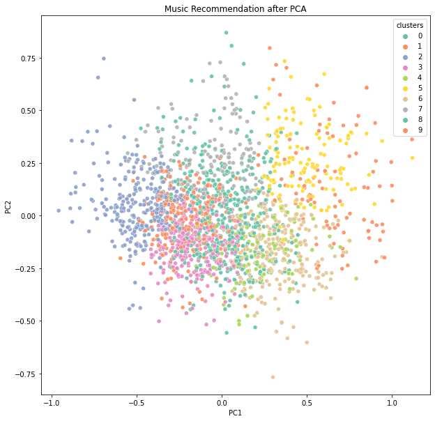
Let's visualize our end clusters after reducing their dimensionality using PCA.

One can find the full code for this project at our GitHub repo for machine learning.

Remarks

The issue is that clusters are not as clearly separated as we expected, but we still see most songs of a cluster are grouped. Increasing the size of the feature vector can address this issue. The feature vector length can be increased by considering audio features for each segment instead of taking the average for the whole song. Here we had a small dataset, but we can try removing outliers on a large dataset, improving the result.

Possible Experiments for further improvements

In the following two sections, we see what further we can do to make a better music recommendation system.

Ordering Songs for Recommendation: We can claim that all songs in a cluster can be considered recommendations for the music. But each song, on average, will have 199 other songs in its cluster, which can be ordered based on songs nearest to the original song. We can calculate this distance using the K-D Tree method. This method is fast for calculating cosine similarity; if we have more data like the popularity of songs and the CTR of the song, we can order them based on that.

Brain think tank: Here, we can improve our music recommendation system using various features, including metadata and audio components. We can use collaborative filtering as discovery is essential considering the current trend. This will be a hybrid approach. These will the steps to build a hybrid approach:

• First, we get vectors of songs using the collaborative filtering method. Let's say we used word2vec on past user listening history and got the vectors.
• As before, we build a new vector using audio features and concatenate one-hot encoding vectors as our metadata. Now, as we generally have a lot of artists and composers, the one-hot encoding vector will be huge, and most will be sparse vectors. This sparsity needs to be reduced using an auto-encoder.
• Finally, we will use this dimensionally reduced vector in K-means. Once we get clusters, ranking can be estimated based on the distance.

This hybrid method covers every feature available and combines the traditional music recommendation system and the present one to give results. 

Possible Interview Questions

• What is the K-means algorithm, and how do we decide the value of k?
• What are the disadvantages of collaborative filtering?
• Why do we need to use audio features and not go with user listening history?
• Suggest some methods by which we can rank the songs.
• Why do we need a music recommendation system?

Conclusion

In this blog, we successfully developed music recommendation systems using an unsupervised learning algorithm, k-means, in Python. This music recommendation system is expected to improve users' retention on the platform and convert them into recurring users.

Enjoy learning. Enjoy algorithms!