Problem-Solving Approaches in Data Structures and Algorithms

This blog highlights some popular problem-solving strategies for solving problems in DSA. Learning to apply these strategies could be one of the best milestones for the learners in mastering data structure and algorithms.

An Incremental approach using Single and Nested loops

One of the simple ideas of our daily problem-solving activities is that we build the partial solution step by step using a loop. There is a different variation to it:

• Input-centric strategy: At each iteration step, we process one input and build the partial solution.
• Output-centric strategy: At each iteration step, we add one output to the solution and build the partial solution.
• Iterative improvement strategy: Here, we start with some easily available approximations of a solution and continuously improve upon it to reach the final solution.

Here are some approaches based on loop: Using a single loop and variables, Using nested loops and variables, Incrementing the loop by a constant (more than 1), Using the loop twice (Double traversal), Using a single loop and prefix array (or extra memory), etc.

Example problems: Insertion Sort, Finding max and min in an array, Valid mountain array, Find equilibrium index of an array, Dutch national flag problem, Sort an array in a waveform.

Decrease and Conquer Approach

This strategy is based on finding the solution to a given problem via its one sub-problem solution. Such an approach leads naturally to a recursive algorithm, which reduces the problem to a sequence of smaller input sizes. Until it becomes small enough to be solved, i.e., it reaches the recursion’s base case.

Example problems: Euclid algorithm of finding GCD, Binary Search, Josephus problem

Problem-solving using Binary Search

When an array has some order property similar to the sorted array, we can use the binary search idea to solve several searching problems efficiently in O(logn) time complexity. For doing this, we need to modify the standard binary search algorithm based on the conditions given in the problem. The core idea is simple: calculate the mid-index and iterate over the left or right half of the array.

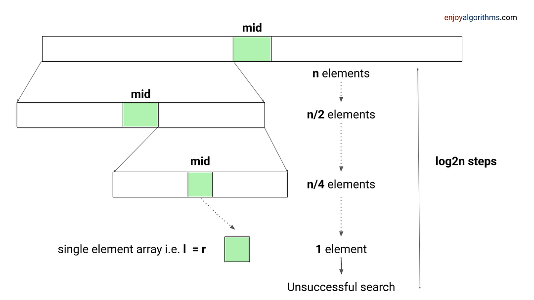
Example problems: Find Peak Element, Search a sorted 2D matrix, Find the square root of an integer, Search in Rotated Sorted Array

Divide and Conquer Approach

This strategy is about dividing a problem into more than one subproblems, solving each of them, and then, if necessary, combining their solutions to get a solution to the original problem. We solve many fundamental problems efficiently in computer science by using this strategy.

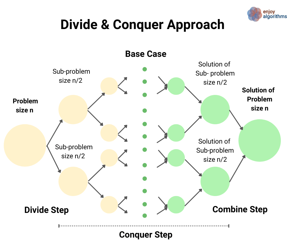
Example problems: Merge Sort, Quick Sort, Median of two sorted arrays

Two Pointers Approach

The two-pointer approach helps us optimize time and space complexity in the case of many searching problems on arrays and linked lists. Here pointers can be pairs of array indices or pointer references to an object. This approach aims to simultaneously iterate over two different input parts to perform fewer operations. There are three variations of this approach:

Pointers are moving in the same direction with the same pace: Merging two sorted arrays or linked lists, Finding the intersection of two arrays or linked lists, Checking an array is a subset of another array, etc.

Pointers are moving in the same direction at a different pace (Fast and slow pointers): Partition process in the quick sort, Remove duplicates from the sorted array, Find the middle node in a linked list, Detect loop in a linked list, Move all zeroes to the end, Remove nth node from list end, etc.

Pointers are moving in the opposite direction: Reversing an array, Check pair sum in an array, Finding triplet with zero-sum, Rainwater trapping problem, Container with most water, etc.

Sliding Window Approach

A sliding window concept is commonly used in solving array/string problems. Here, the window is a contiguous sequence of elements defined by the start and ends indices. We perform some operations on elements within the window and “slide” it in a forward direction by incrementing the left or right end.

This approach can be effective whenever the problem consists of tasks that must be performed on a contiguous block of a fixed or variable size. This could help us improve time complexity in so many problems by converting the nested loop solution into a single loop solution.

Example problems: Longest substring without repeating characters, Count distinct elements in every window, Max continuous series of 1s, Find max consecutive 1's in an array, etc.

Transform and Conquer Approach

This approach is based on transforming a coding problem into another coding problem with some particular property that makes the problem easier to solve. In other words, here we solve the problem is solved in two stages:

1. Transformation stage: We transform the original problem into another easier problem to solve.
2. Conquering stage: Now, we solve the transformed problem.

Example problems: Pre-sorting based algorithms (Finding the closest pair of points, checking whether all the elements in a given array are distinct, etc.)

Problem-solving using BFS and DFS Traversal

Most tree and graph problems can be solved using DFS and BFS traversal. If the problem is to search for something closer to the root (or source node), we can prefer BFS, and if we need to search for something in-depth, we can choose DFS.

Sometimes, we can use both BFS and DFS traversals when node order is not required. But in some cases, such things are not possible. We need to identify the use case of both traversals to solve the problems efficiently. For example, in binary tree problems:

• We use preorder traversal in a situation when we need to explore all the tree nodes before inspecting any leaves.
• Inorder traversal of BST generates the node's data in increasing order. So we can use inorder to solve several BST problems.
• We can use postorder traversal when we need to explore all the leaf nodes before inspecting any internal nodes.
• Sometimes, we need some specific information about some level. In this situation, BFS traversal helps us to find the output easily.

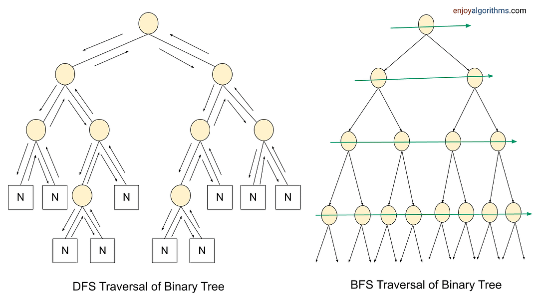
To solve tree and graph problems, sometimes we pass extra variables or pointers to the function parameters, use helper functions, use parent pointers, store some additional data inside the node, and use data structures like the stack, queue, and priority queue, etc.

Example problems: Find min depth of a binary tree, Merge two binary trees, Find the height of a binary tree, Find the absolute minimum difference in a BST, The kth largest element in a BST, Course scheduling problem, bipartite graph, Find the left view of a binary tree, etc.

Problem-solving using the Data Structures

The data structure is one of the powerful tools of problem-solving in algorithms. It helps us perform some of the critical operations efficiently and improves the time complexity of the solution. Here are some of the key insights:

• Many coding problems require an effcient way to perform the search, insert and delete operations. We can perform all these operations using the hash table in O(1) time average. It's a kind of time-memory tradeoff, where we use extra space to store elements in the hash table to improve performance.
• Sometimes we need to store data in the stack (LIFO order) or queue (FIFO order) to solve several coding problems. 
• Suppose there is a requirement to continuously insert or remove maximum or minimum element (Or element with min or max priority). In that case, we can use a heap (or priority queue) to solve the problem efficiently.
• Sometimes, we store data in Trie, AVL Tree, Segment Tree, etc., to perform some critical operations efficiently. 

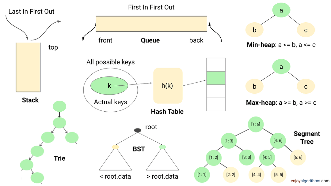
Example problems: Next greater element, Valid Parentheses, Largest rectangle in a histogram, Sliding window maximum, kth smallest element in an array, Top k frequent elements, Longest common prefix, Range sum query, Longest consecutive sequence, Check equal array, LFU cache, LRU cache, Counting sort

Dynamic Programming

Dynamic programming is one of the most popular techniques for solving problems with overlapping or repeated subproblems. Here rather than solving overlapping subproblems repeatedly, we solve each smaller subproblems only once and store the results in memory. We can solve a lot of optimization and counting problems using the idea of dynamic programming.

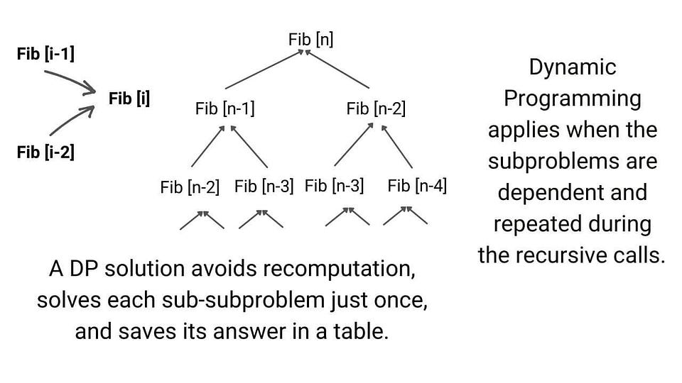
Example problems: Finding nth Fibonacci, Longest Common Subsequence, Climbing Stairs Problem, Maximum Subarray Sum, Minimum number of Jumps to reach End, Minimum Coin Change

Greedy Approach

This solves an optimization problem by expanding a partially constructed solution until a complete solution is reached. We take a greedy choice at each step and add it to the partially constructed solution. This idea produces the optimal global solution without violating the problem’s constraints.

• The greedy choice is the best alternative available at each step is made in the hope that a sequence of locally optimal choices will yield a (globally) optimal solution to the entire problem.
• This approach works in some cases but fails in others. Usually, it is not difficult to design a greedy algorithm itself, but a more difficult task is to prove that it produces an optimal solution.

Example problems: Fractional Knapsack, Dijkstra algorithm, The activity selection problem

Exhaustive Search

This strategy explores all possibilities of solutions until a solution to the problem is found. Therefore, problems are rarely offered to a person to solve the problem using this strategy.

The most important limitation of exhaustive search is its inefficiency. As a rule, the number of solution candidates that need to be processed grows at least exponentially with the problem size, making the approach inappropriate not only for a human but often for a computer as well.

But in some situations, there is a need to explore all possible solution spaces in a coding problem. For example: Find all permutations of a string, Print all subsets, etc.

Backtracking

Backtracking is an improvement over the approach of exhaustive search. It is a method for generating a solution by avoiding unnecessary possibilities of the solutions! The main idea is to build a solution one piece at a time and evaluate each partial solution as follows:

• If a partial solution can be developed further without violating the problem’s constraints, it is done by taking the first remaining valid option at the next stage. (Think!)
• Suppose there is no valid option at the next stage, i.e., If there is a violation of the problem constraint, the algorithm backtracks to replace the partial solution’s previous stage with the following option for that stage. (Think!)

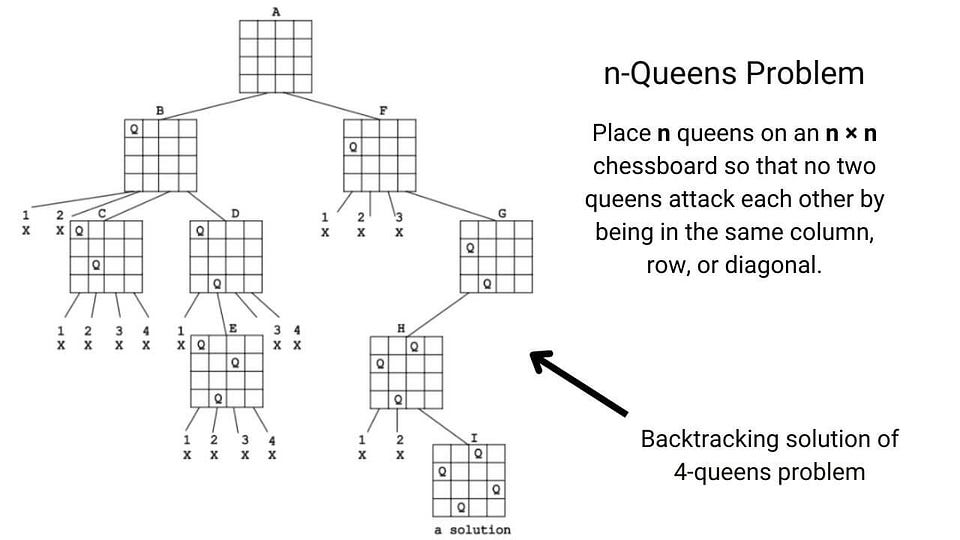
In simple words, backtracking involves undoing several wrong choices — the smaller this number, the faster the algorithm finds a solution. In the worst-case scenario, a backtracking algorithm may end up generating all the solutions as an exhaustive search, but this rarely happens!

Example problems: N-queen problem, Find all k combinations, Combination sum, Sudoku solver, etc.

Problem-solving using Bit manipulation and Numbers theory

Some of the coding problems are, by default, mathematical, but sometimes we need to identify the hidden mathematical properties inside the problem. So the idea of number theory and bit manipulation is helpful in so many cases.

Sometimes understanding the bit pattern of the input and processing data at the bit level help us design an efficient solution. The best part is that the computer performs each bit-wise operation in constant time. Even sometimes, bit manipulation can reduce the requirement of extra loops and improve the performance by a considerable margin.

Example problems: Reverse bits, Add binary string, Check the power of two, Find the missing number, etc.

Hope you enjoyed the blog. Later we will write a separate blog on each problem-solving approach. Enjoy learning, Enjoy algorithms!