Soil Fertility Prediction Using Machine Learning

Agricultural production has seen tremendous growth in the last couple of decades with advancements in technologies. To ease the farming process, we are now using Smart Farming techniques using machine learning and data science, which are helping in increasing the quantity and quality simultaneously.

As one of the smart use cases of machine learning in farming, we will be learning the implementation steps of gradient boosting algorithm to predict soil fertility in this article.

Problem Background 

Machine Learning has become a tool used in almost every task that requires estimation. The non-technical sector, such as agriculture, has also benefited from these techniques. This applies to predicting soil fertility using specific properties that vary from region to region. Traditional methods such as crop rotation, incorporating cover crops, and adding organic matter to soil have helped this sector yield more crops. Still, they do not utilize the available domain knowledge by 100%.

Soil fertility prediction does not promise us more yield, but it does promise us the extent to which our incorporated methods have improved the soil quality. Soil fertility prediction will help to condense the difficulties faced by the farmers and act as a medium to bid the agriculturalists efficient evidence required to get better yield.

The task of predicting soil fertility is not new to Machine Learning. Experts and consultants have tried several possibilities to use different machine learning methods to predict it. Classification algorithms have proven sufficient accuracy to deal with such a problem. ML algorithms such as k-NN, DTs, SVM, and, Random Forests have been used for different case studies on soil fertility. In this article, we will be using Gradient Boosting and guide you to understand: why we are using gradient boosting?

Gradient Boosting Classifier for Soil Fertility Prediction

Gradient Boosting falls under the category of Ensemble Methods. Ensemble methods incorporate a team of classifiers and vote them while testing their performance. These methods usually reduce the variance of the classifier. The main advantage of ensembling is that it is unlikely for all the classifiers to make the same error. In fact, as long as every error is made by a minority of the classifiers, proper classification can be achieved.

Gradient Boosting Connection-Tree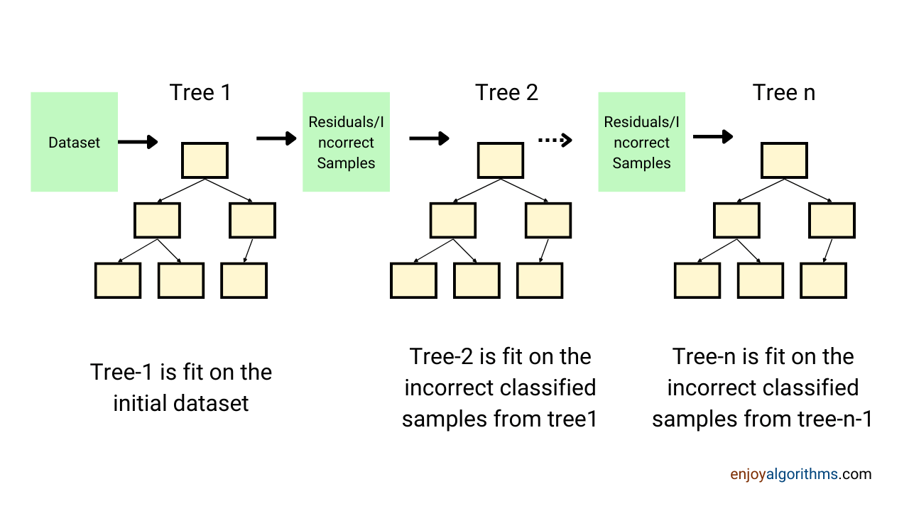

In Gradient Boosting, each predictor tries to improve on its ancestor by reducing the errors. Instead of fitting a model on the data to each iteration, Gradient Boosting essentially fits a new model to the previous ancestor model's residual errors. For every instance, while training, it estimates the residuals for that instance in terms of the log of odds. Once done, it builds a new Decision Tree that tries to predict the residuals estimated by the previous estimator. This is the main difference between Gradient Boosting Methods (GBM) and Random Forests (RF). 

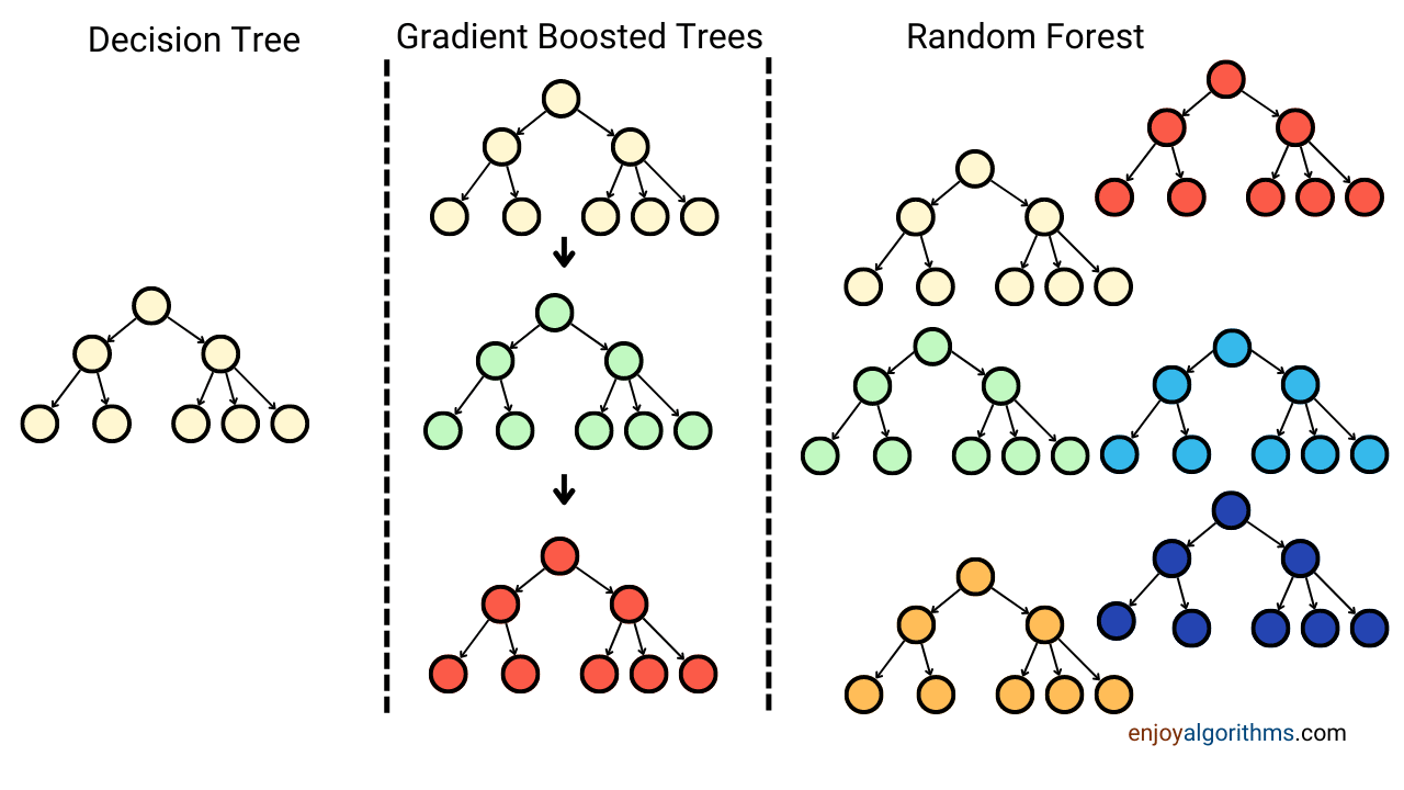
GBMs build an ensemble of shallow and weak sequential trees with each tree learning and improving on the prior, while random forests only ensemble independent trees. Using empirical results, it can be argued that the accuracy of Gradient Boosting can be hard to beat, although this approach is computationally expensive.

Let’s quickly move towards the core part of this article, where we will be guiding you to make your ML model that can predict the fertility of the soil.

Steps to implement the solution

Step 1: Data Collection

Various datasets can be found on the internet very easily. Government sectors also release their dataset in the public domain. State-wise, data from India can be downloaded from the farmer’s portal. Based on the above portal, a sample dataset can be used from here. We will be using this dataset in this article.

Step 2: Dataset explanation

The dataset contains sixteen different attributes. An explanation of every attribute is given in the table below.

Attribute Explanation

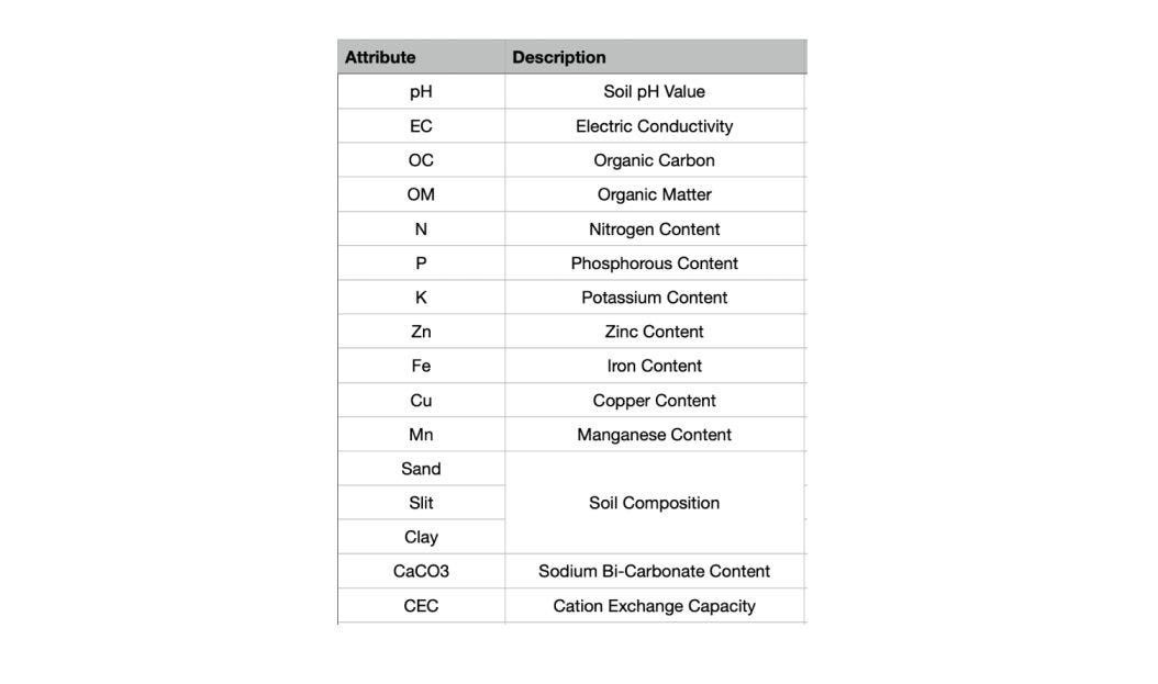
Sampled instances of the dataset

A snippet of the data can be seen by printing the dataframe sample.

Step 3: Data Pre-processing

With the seaborn library's help, we can plot the correlation between the dataset attributes. If we observe the below plot, attributes OC and OM are highly correlated, so in the final set of features used for training the model, we can select any one of them.

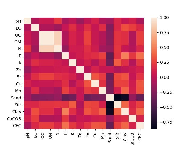
We can have these input features in the final set: pH, EC, OC, N, P, K, Zn, Fe, Cu, Mn, Sand, Silt, Clay, CaCO3, and CEC. At the same time, the output feature vector is the decision vector formed from the last column. All these features have different ranges. So using the MinMaxScaler() of Sklearn’s preprocessing tool, all the attributes can be scaled in the range of [0,1]. Alternatively, MaxAbsScaler() can be used to scale in the [-1,1] range. Using labelEncoder(), decision column (last column) of the dataset can be converted into numerical value (0 & 1). 

This dataset can be split into two sets:

1. Train Data 
2. Validation Data: A validation set will be used to tune the hyperparameters.

Step 4: Model Formation

Setting up the algorithm 

• From the module sklearn.ensemble import the algorithm GradientBoostingClassifier()to build a model. Certain hyperparameters need to be tuned efficiently. 
• Take the learning rate to be higher than usual (say 0.2-0.25 instead of 0.1).
• Chose a maximum depth (play around with values between 5–10), similarly play with the regularization parameter (alpha: 1e-3 to 1e-2 in steps of 1e-1)

model = GradientBoostingClassifier(n_estimators=100, learning_rate=1.0,
...     max_depth=1, random_state=0).fit(X_train, y_train)

training & fitting Algorithm with training Dataset can be fitted on the developed model using the model.fit(train_feature, output)

Step 5: Evaluation of developed model

Model Score: This gives the mean accuracy of the given test data and labels. For the above model, model.score(testX, testy) will give you the model's average score.

Confusion Matrix: The confusion matrix can be imported from the metrics module of the sklearn library. The test set can be used to compare the predicted output and the ground truth.

Companies Case Studies

The use of Machine Learning technology in the area of agriculture can revolutionize the economy. With the consistently decreasing agricultural area, the prime need that yield should be maximized with the limited land. Big corporations such as Mineral, Cool Planet, and AgSolver are working actively on improving soil health by considering various factors and developing soil test kits and strategies to deploy them. 

Google’s Mineral

Alphabet’s X lab, a former Google division that launched the Waymo self-driving car unit and other ambitious projects, has taken the wraps off its latest “moonshot”: a computational agriculture project called Mineral.

According to the Mineral’s lead, Elliott Grant, “Mineral project is focused on sustainable food production and farming with the help of advanced technologies of artificial intelligence, robotics, machine learning and simulations at an immense scale.”

Cool Planet

Cool Planet is an agricultural technology company mainly focused on soil health solutions. It uses advanced technologies for predicting the fertility of the soil. It has acquired $20.3 million of Series A funding. The company’s two largest existing investors, Agustín Coppel and North Bridge Venture Partners, led the investment.

Possible Interview Questions

• Is soil fertility prediction a multi-class classification problem? If No, can we convert it to the same?
• Which algorithms did you try along with boosting algorithm? On what basis did you select this algorithm?
• How boosting algorithms is connected with the random forest?
• Do you think your results are the best? What improvements you can suggest?
• Explain the boosting algorithm.

Conclusion

Machine Learning technology helps farmers make the farming process easy and ensures the yield's better quality and quantity. Famers mainly rely upon ML to automatically increase the quality and quantity of products, automatically detect the plant's diseases, the presence of weeds, and livestock management. Many big corporations are trying to improve the yield with satellite data and ground measured data. Soil fertility prediction is one of the techniques that identifies whether any land is suitable for a particular crop or not.

In this article, we have formed our soil fertility prediction model that can sense soil fertility based on attribute measurements. Based on this prediction, farmers can decide whether they should choose land for agricultural purposes or not. I hope you have enjoyed this use case.

Enjoy Learning, Enjoy Algorithms!