Hands-on Methods for Structured Data Pre-Processing

Introduction

Companies are collecting tons of data, and with this, the need for processed data is highly increasing. In the previous blogs, we have seen the following data preprocessing techniques in theory:

• Feature Selection
• Feature Quality Assessment
• Feature Sampling
• Feature Reduction

In this blog, we will do hands-on on all these preprocessing techniques. We will use different datasets for demonstration and briefly discuss the intuition behind the methods. So let's start without any further delay.

Feature Selection

Selecting the appropriate feature for data analysis requires the knowledge of feature selection methods and some domain knowledge. Combining both allows us to choose the optimum features necessary for tasks. We will discuss one technique from each feature selection method. Let's first see the types of feature selection methods:

Wrapper Methods

The wrapper method requires a machine-learning algorithm to find the optimum features. This method generally has a high computational time. There are many methods for finding the significant features, but we will confine ourselves to Sequential Feature Selector (for step-wise selection). This is a greedy algorithm that sequentially checks the model's performance with each feature and sequentially adds to the features.

import pandas as pd
import numpy as np
from mlxtend.feature_selection import SequentialFeatureSelector
from sklearn.linear_model import LinearRegression


features = boston_house_price.iloc[:,:13]
target = boston_house_price.iloc[:,-1]
SFS = SequentialFeatureSelector(LinearRegression(),
                                k_features=7,
                                forward=True,
                                floating=False,
                                scoring = 'r2')


SFS.fit(features, target)
SFS_results = pd.DataFrame(SFS.subsets_).transpose()
SFS_results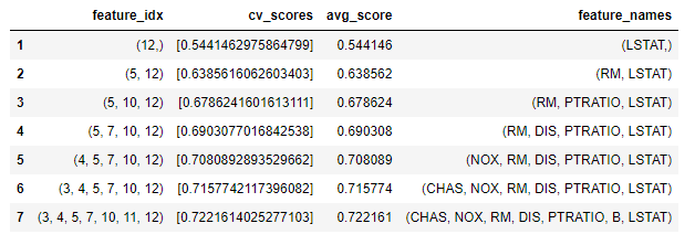

Filter Methods

Filter methods are a set of statistical techniques required for measuring the importance of features in a dataset. It includes Correlation, Chi-Square test, information gain, etc. These methods are comparatively faster in terms of time complexity. Let's implement correlation as a feature selection criteria:

import seaborn as sns
import matplotlib.pyplot as plt

correlation = boston_house_price.corr()

plt.figure(figsize= (15,12))
SNS.heatmap(correlation, annot=True)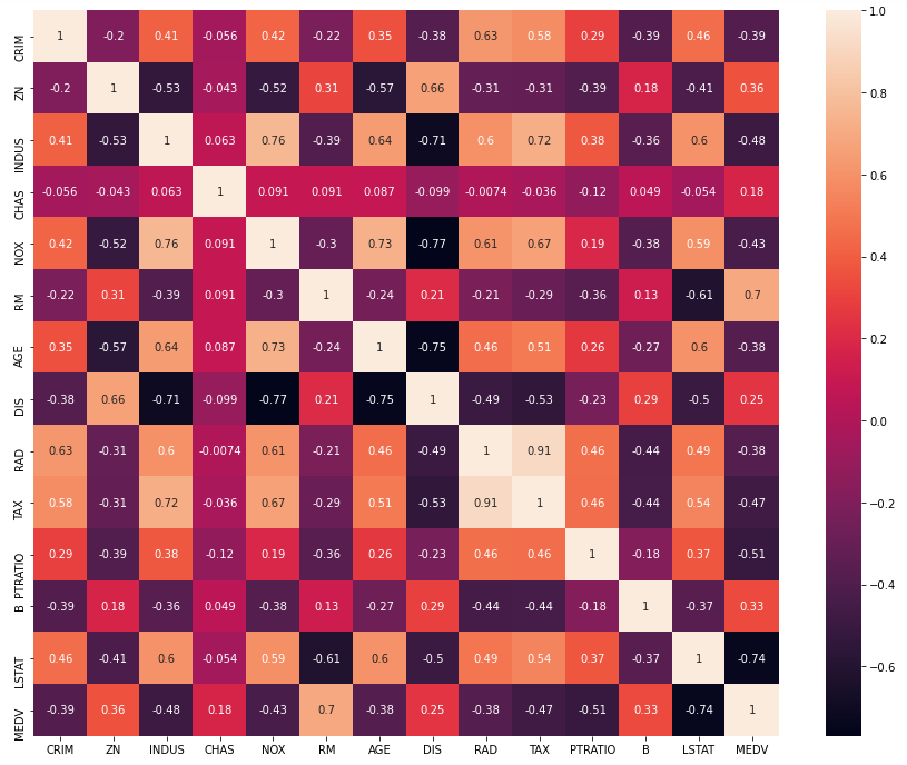

RAD and TAX are highly correlated, and therefore, we can remove one with a low value of absolute correlation with the target variable (MEDV). "RAD" can be removed. Also, we can set a threshold value of the absolute correlation to remove the less informative features. For instance, if we select 0.40 correlation as a feature selection criteria for the modeling, we are left with 'INDUS,' 'NOX,' 'RM,' 'TAX,' 'PTRATIO,' 'LSTAT.' as the final set of features.  

Embedded Methods

Embedded methods combine the qualities of Filter and Wrapper methods. It works by iteratively building the models while also evaluating their performance. Based on performance, the best set of parameters is chosen. Again, there are many techniques within embedded methods, but we will use Random Forest Feature Importance. Let's implement RF Feature Importance for selecting the optimum features:

from sklearn.ensemble import RandomForestRegressor

rfr = RandomForestRegressor(n_estimators=1300)
rfr.fit(features, target)

importance = rfr.feature_importances_

importance_df = pd.DataFrame({"Features": features.columns, "Importance":importance})
importance_df = importance_df.sort_values("Importance")

plt.bar(importance_df["Features"], importance_df["Importance"])
plt.show()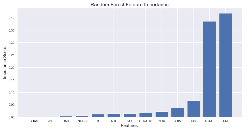

From the above plot, we can conclude 'RM,' 'LSTAT,' 'DIS,' 'CRIM,' and 'NOX' as the optimal features in the analysis. Embedded methods fall between the filter and wrapper methods in time complexity. 

We could have discussed more techniques from each method, but we will revisit this topic in a separate blog on Feature Selection techniques. Let's move on to the feature quality assessment.

Feature Quality Assessment

This section deals with the quality of data. Data is prone to noise, human errors, scaling errors, and reading errors. Such errors induce inconsistency in the collected data. It is recommended to process the data to remove these inconsistencies, and we will do the same on the Advanced Regression house price dataset. 

Missing Values

Missing values are inevitable in raw data. Sometimes, sensors don't work the way we want, or it could be a case where data isn't available, and such cases result in the presence of missing values in the data. Let's look at ways of treating the missing values in the data.

Row Elimination

Sometimes, only a few rows have missing values. Removing 1 to 10% of data doesn't make significant differences; however, in time-series data where sequential data points are collected over a fixed period, this method can cause problems. 

Imputation

In this method, we replace the missing values with specific imputed values. The imputation methods are different for numerical and categorical features. It is recommended to separate the numeric and categorical features beforehand. Afterward, we will break the imputation problem as the imputation of categorical features and numerical features. 

We are going to apply some imputation techniques to the given dataset. Take a look at the dataset:

import pandas as pd

purchase = pd.read_csv('purchase.csv')
print(purchase)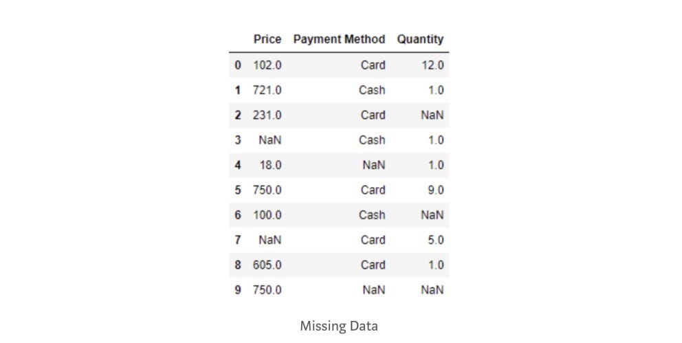

Imputation methods for numerical variables:

• Mean/Median Imputation

# Mean Imputation
purchase['Price']=purchase['Price'].fillna(purchase['Price'].mean())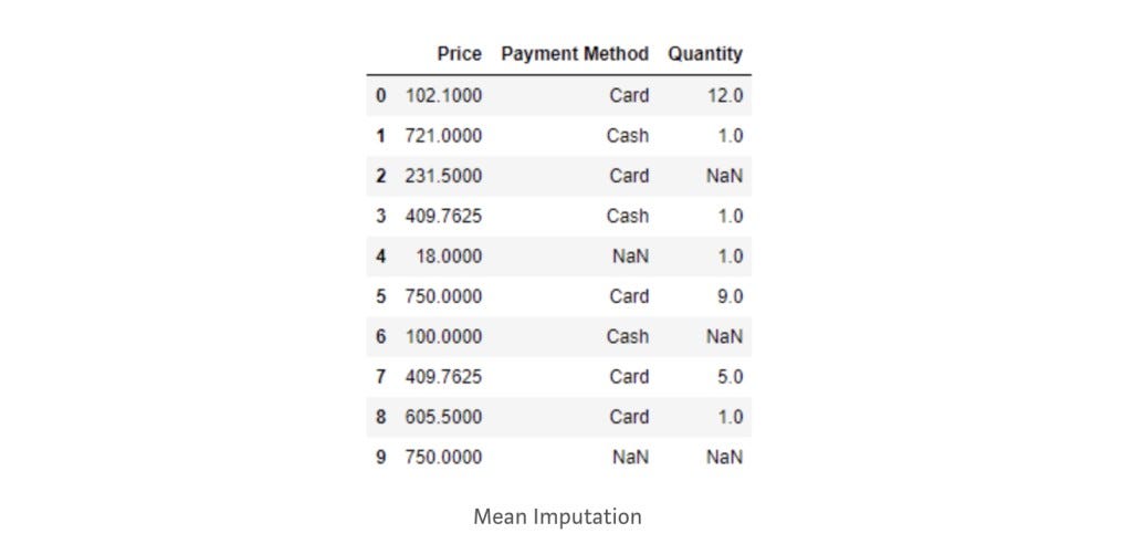

# Median Imputation
purchase['Price']=purchase['Price'].fillna(purchase['Price'].median())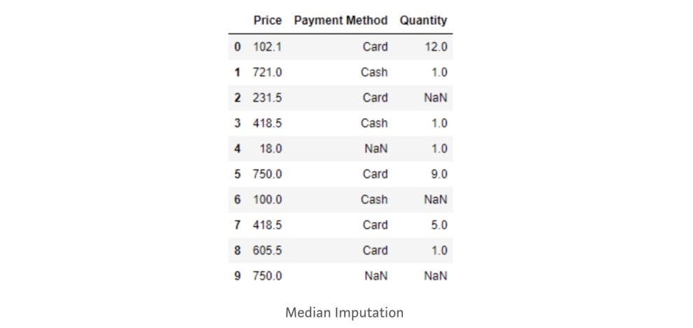

• Forward Fill/Backward Fill

# Forward Fill
purchase["Price"].fillna(method='ffill', inplace=True)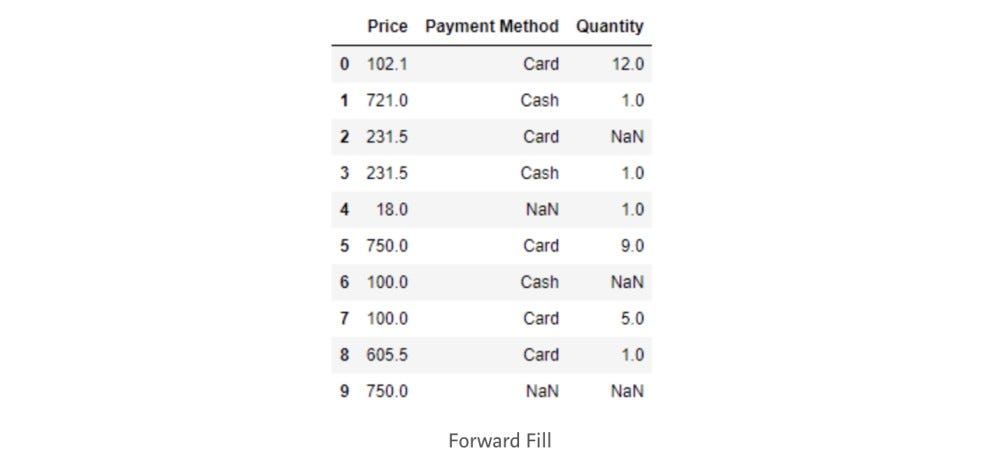

# Backward Fill
purchase["Price"].fillna(method='bfill', inplace=True)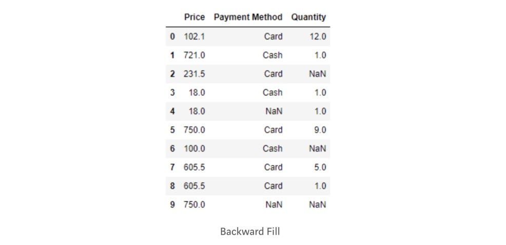

• Interpolation

# Linear Interpolation
purchase["Price"]= purchase["Price"].interpolate()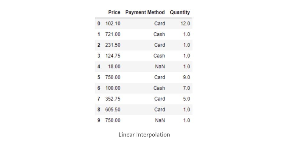

Imputation methods for categorical variables:

• Frequent Category Imputation

purchase['Payment Method'] = purchase['Payment Method'].fillna(purchase['Payment Method'].mode().iloc[0])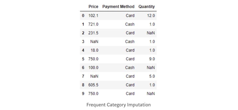

• Adding a new category as "Missing."

purchase['Payment Method'] = purchase['Payment Method'].fillna('Missing')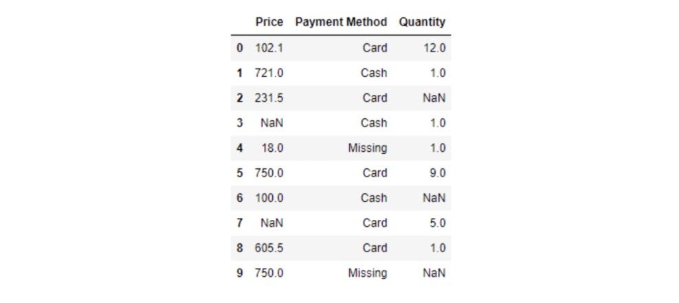

Outlier

Outliers are the abnormal readings or data points present in the dataset. They are highly distinguishable and need to be removed since they can cause severe problems during the model building phase. There are two ways of detecting an outlier from the dataset:

• Using Statistical Method
• Using Machine Learning Algorithms

Let's look at some statistical methods available for the removal of outliers from the data:

Inter Quartile Range (IQR)

If you are unfamiliar with Quartile, please have a look at this. Inter Quartile Range is nothing but the difference between the third and first Quartile. More formally:

IQR = Q3 - Q1

Data points above Q3 + 1.5 IQR and below Q1 – 1.5IQR are treated as outliers. Let's implement this in our dataset:

import pandas as pd

temperature = pd.read_csv('temp.csv') # temperature is a dataframe
temperature.head()

Q1 = temperature['Temperature'].quantile(0.25)
Q3 = temperature['Temperature'].quantile(0.75)

IQR = Q3 - Q1
upper_limit = Q3 + 1.5 * IQR
lower_limit = Q1 - 1.5 * IQR

anomaly = temperature[(temperature['Temperature'] > upper_limit) | (temperature['Temperature'] < lower_limit)]
print(anomaly)

Standard Deviation

This approach is relatively simple and effective as it only requires the computation of mean and standard deviation to calculate the upper and lower bounds. Any value within these bounds is a safe value and otherwise anomaly. Let's implement this approach:

upper_bound = temperature['Temperature'].mean() + 3*temperature['Temperature'].std()

lower_bound = temperature['Temperature'].mean() - 3*temperature['Temperature'].std()

anomaly = temperature[(temperature['Temperature'] > upper_bound) | (temperature['Temperature'] < lower_bound)]
print(anomaly)

Duplicate Values

Duplicate values can be present due to various factors. Such data points can lead to model bias. Let's remove the duplicate rows from the dataset:

temperature.drop_duplicates(inplace=True)

Data Sampling

Data Sampling is a statistical technique used to manipulate and examine a representative subset of the original dataset. It helps identify and visualize trends and patterns while also reducing computational efforts. Following are some frequently used data sampling methods:

Upsampling/Downsampling

Upsampling and Downsampling techniques are generally used in Classification problems to address the class imbalance. It simply works by reducing or increasing the samples from the majority or minority classes depending on the type of Sampling used. Let's apply them one by one:

Consider a binary classification with unbalanced labels (Class1 has more samples than Class2). We aim to downsample the data points for Class_1 to eliminate the class imbalance.

Downsampling:

# Downsampling
import numpy as np
downsampled = np.random.choice(Class_1, size=Class_0, replace=False)

After Downsampling

Upsampling:

# Upsampling
import numpy as np
downsampled = np.random.choice(Class_0, size=Class_1, replace=True)

After Upsampling

Stratified Sampling

Stratified Sampling is the most commonly used sampling technique in classification problems to make the test and training dataset. This method samples the data such that classes are divided into homogenous sub-groups, maintaining the same proportions. These homogenous sub-groups are also known as strata.

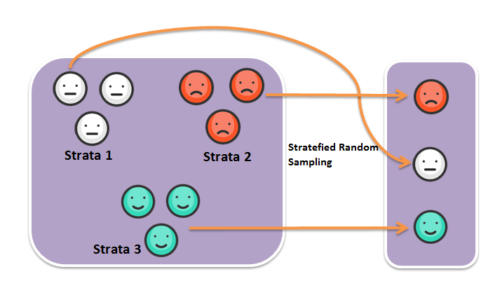
Source: Data Science Made Simple

#Load the dataset
dress_code = pd.read_csv('Clothing Color.csv')
print(dress_code)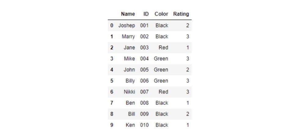

Let's select the stratified samples of the above dataset based on the dress color code. As we can see, 50% of participants are wearing Black, 30% of participants are wearing Green, and the rest 20% of participants are wearing Red dresses. Our stratified sampled dataset must retain this proportion. Let's implement stratified Sampling:

# Stratified Sampling
dress_code.groupby('Color', group_keys=False).apply(lambda x: x.sample(frac=0.6))

Simple Random Sampling

As the name suggests, it is a statistical sampling method where each data point in a dataset has an equal probability of being selected in a dataset. This sampling results in an unbiased representation of a group. Let's apply random SamplingSampling in the dress color code dataset:

# Random Sampling
dress_code.sample(n=6, random_state=1)

Feature Reduction

Nowadays, firms collect a lot of features for the analysis but using all of them for modeling is not feasible since this will come at a computational cost, and dimensionality reduction addresses this problem by reducing the number of features and keeping them intact with the same level of information. 

Following are some techniques available for reducing the dimensionality of the dataset. Let's discuss them along with their application:

Principal Component Analysis (PCA)

PCA is a statistical dimensionality reduction method used to reduce the number of dimensions from a larger dataset. This feature reduction technique comes at the cost of minimal information loss, but this can save a lot of computational efforts and make the visualization better. Machine learning algorithms are much easier to implement with reduced features. Let's implement PCA to the dataset. 

import pandas as pd
transaction_data = pd.read_csv('creditcard.csv')

transaction_feature = transaction_data.iloc[:,:-2]

transaction_feature.head()

Transactional Data

Generally, we first normalize the dataset and then apply PCA, but features are already scaled in our case, so normalization is not required.

from sklearn.decomposition import PCA

pca = PCA()
transaction_feature = pca.fit_transform(transaction_feature)

explained_variance = pca.explained_variance_ratio_
print(explained_variance*100)

Percentage Variance captured by each feature.

The first 17 Principal Components cover 85% information (variance) of the original dataset. Let's reduce the dataset to 17 features:

pca = PCA(n_components=17)

reduced_features = pca.fit_transform(transaction_feature)

reduced_features = pd.DataFrame(reduced_features)

Initially, we had 28 features, and we reduced the number of features to 17 at the cost of 15% information loss. 

t-SNE

t-Distributed Stochastic Neighbor Embedding (t-SNE) is another dimensionality reduction technique. It is specifically used for the visualization of high-dimensional data. Moreover, It is computationally expensive, and hence, there are some severe limitations to this technique. For instance, using a "Second dimensionality reduction technique" is highly advisable in some cases of very high dimensional data. Let's apply t-SNE to our dataset:

from sklearn.manifold import TSNE

tsne = TSNE(n_components=3, verbose=1, perplexity=40, n_iter=300)

tsne_results = tsne.fit_transform(reduced_features)

Conclusion

In this article, we have demonstrated the methodology of data preprocessing techniques. We looked at different feature selection methods and applied them to the Boston house price dataset. Further, we looked at some feature quality assessment techniques where we discussed and used Missing value imputation techniques and Outlier Detection techniques. Moving onwards, we also observed some sampling methods and dimensionality reduction techniques and applied them to a dataset. We hope you enjoyed the article.

Enjoy Learning, Enjoy Algorithms!