Word Vector Encoding in NLP (Make Machines Understand Text)

Natural Language Processing (NLP) is a broad field that covers a lot of applications related to text and speech like sentiment analysis, named entity recognition, language modeling, text summarization, speech recognition, etc. However, before working on any of these applications, one needs to know the basics of word vector representation. 

In our previous article (here), we learned about the different pre-processing techniques for the text data, including,

• Lowercasing the words.
• Hyperlink, Punctuation, and stopwords removal.
• Spelling correction and tokenization.
• Stemming and Lemmatization
• Text exploratory analysis: Visualizing most frequent words, WordCloud, and visualizing the sentiment of words.

But, there is still something essential and not discussed there. Unlike humans, machines don’t understand words and the semantic context present in them. Computers only understand numbers, not text. So we need to convert our processed text into a format that computers can understand.

To make this possible, the concept of Word Embeddings was introduced in 2013 by Tomas Mikolov at Google. Ever since the word embeddings were introduced, they turned the impossible tasks in NLP possible. Let’s dive deeper and understand: How do word embeddings work?

Key takeaways from this blog

1. What is word embedding?
2. Techniques to embed the words: One-hot encoding, Word2Vec, TF-IDF, and Bag of Words.
3. Basic implementation of all these embeddings.
4. Advantages of TF-IDF.

Word Embeddings

Word Embedding is a term used in NLP for the representation of words for text analysis. Words are encoded in real-valued vectors such that words sharing similar meaning and context are clustered closely in vector space. Word embeddings can be obtained using language modeling and feature learning techniques where words or phrases from the vocabulary are mapped to vectors of real numbers. In simple terms, word embeddings are a form of word representation that connects the human understanding of language to that of a machine. Word embeddings are crucial for solving NLP problems.

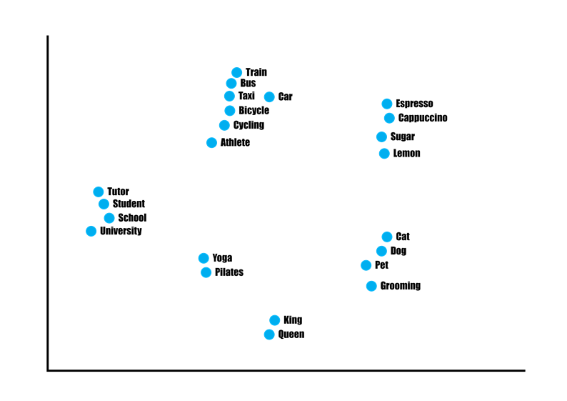
Source: Predictive Hacks

Several methods can be used to perform the task of word embeddings. However, the idea behind all of them is common, that is, to capture most of the context and semantic information present in the text. We must ask ourselves,

If there are multiple methods to perform word embeddings, then when to choose which method?

In the end, one method will outperform the others, but choosing the optimal word embedding for the project is decided based on an empirical try-and-fail approach. 

Let’s look at some reliable Word embedding approaches and their limitations. For this task, we will be using the Coronavirus Tweets NLP Text Classification dataset for demonstration. We have already applied some text pre-processing steps in our previous blog on text mining. We will continue building the word embedding on the same pre-processed data. Feel free to visit the text mining blog for a quick recap.

One Hot Encoding

In NLP, One hot encoding is a vector representation of words in a “vocabulary”. Each word in the vocabulary is represented by a vector of size ’n’, where ’n’ is the total number of words in the vocabulary. For instance, if a vocabulary contains 10 words, then the vector corresponding to each word will have a size of 10, and that too with binary values like ‘0’ and ‘1’.

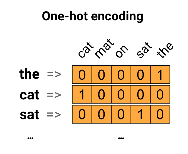
Source: TensorFlow

Let’s implement One Hot Encoding for the first 10 tokens in the vocabulary:

from sklearn.preprocessing import OneHotEncoder
from sklearn.preprocessing import LabelEncoder
label_encoder = LabelEncoder()
integer_label_encoded = label_encoder.fit_transform(tokens[1:10])
label_encoded = integer_label_encoded.reshape(len(integer_label_encoded), 1)
onehot_encoder = OneHotEncoder(sparse=False)
onehot_encoded = onehot_encoder.fit_transform(label_encoded)
print(onehot_encoded)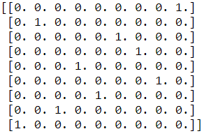

One Hot Encoded Vectors

Pros & Cons of One Hot Encoding:

Pros:

• Highly intuitive and straightforward to compute

Cons:

• Memory Inefficient (Requires very high memory when vocabulary is large)
• Word Similarity Context is not defined. Suppose we implemented one word with vector V1 and another word with another vector V2. From the above definition of word-embedding, these two vectors will be perpendicular to each other (Think!) and considered independent. But two words can be dependent.

Word2Vec

In 2013, Tomas Mikolov came up with state-of-the-art Word2Vec word embedding. If you are familiar with the concept of neural networks, you mi

It is a two-layer neural network that processes the text by vectorizing words. Input for Word2Vec is a corpus, and the output is a set of feature vectors representing the words in that corpus. Embeddings generated by Word2Vec have proven to be successful on a variety of NLP tasks.

Word2Vec model has two methods for learning representations of words:

• Continuous Bag-of-Words Model (CBOW): which predicts the middle word based on surrounding context words. The context consists of a few words before and after the current (middle) word. This architecture is called a bag-of-words model as the order of words in the context is not essential.
• Continuous Skip-gram Model: It predicts words within a certain range before and after the current word in the same sentence.

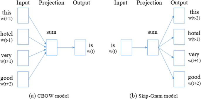
Word2vec is similar to an autoencoder, encodes each word in a vector, and trains words against other neighboring words in the input corpus. Word2Vec either uses the context to predict a target word (CBOW) or uses a word to predict a target context, called skip-gram. Skip Gram generally performs better on large datasets.

For demonstration, we will implement both of them in our corpus and will compare the cosine similarity scores.

Cosine similarity is a measure of similarity between two non-zero vectors. Measuring the similarity between word vectors allows us to measure the closeness of words represented by those vectors.

import gensim
from gensim.models import Word2Vec
CBOW = gensim.models.Word2Vec([token_list], vector_size=10, window=5, min_count=1, workers=4)
print("Cosine similarity between 'Market' " + "and 'Stock' - Continuous Bag of Word : ", CBOW.wv.similarity('market', 'stock'))

import gensim
from gensim.models import Word2Vec
CSG = gensim.models.Word2Vec([token_list], vector_size=10, window=5, min_count=1, workers=4, sg=1)
print("Cosine similarity between 'Market' " + "and 'Stock' - Skip Gram: ", CSG.wv.similarity('market', 'stock'))

Both Word2Vec models performed well on our corpus!

Pros & Cons of Word2Vec:

Pros:

• Highly intuitive and easy to understand
• Requires low pre-processing
• Retains the context

Cons:

• No explicit explanation of the context
• Relatively difficult to train

TF-IDF

TF-IDF is an information retrieval method that relies on Term Frequency (TF) and Inverse Document Frequency (IDF) to measure the importance of a word in a document. A survey conducted in 2015 showed that 83% of text-based recommender systems in digital libraries use TF-IDF.

What makes TF-IDF so effective?

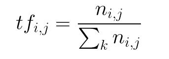
In a document, not all words have equal significance, and therefore, one can assign weights to these words based on their term frequency and inverse document frequency. Words like ‘the’, ‘and’, ‘he’ etc., appear very frequently, but they don’t carry any weightage. The TF-IDF weightage of a word in the document is calculated as the product of term frequency and inverse document frequency of that word. This product is higher for rare terms in the document and relatively lower for commonly used words.

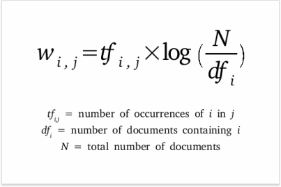
• Term Frequency

Term Frequency is the number of times a specific word appeared in the document divided by the total number of words in the document.

• Inverse Document Frequency

The inverse document frequency measures whether a term is common or rare in a given document. It is obtained by dividing the total number of documents by the number of documents containing the term in the corpus.

Once these two metrics have been calculated, they can be combined to get a new measure: the term frequency × the inverse document frequency. This product reflects how important a word is with respect to a given document in a corpus of documents.

Implementing TF-IDF

from nltk.stem.porter import PorterStemmer
from sklearn.feature_extraction.text import TfidfVectorizer
def tokenize(text):
    tokens = nltk.word_tokenize(text)
    stems = []
    for item in tokens:
        stems.append(PorterStemmer().stem(item))
    return stems
tfidf = TfidfVectorizer(tokenizer=tokenize, stop_words='english')
tfs = tfidf.fit_transform(tweets["Text"])
# to visualize the formed TF-IDF matrix
tfs.toarray()

Pros & Cons of TF-IDF:

Pros:

• Easy to understand
• Easy to compute
• Considers other documents

Cons:

• Requires high memory for feature creation when the dataset is large
• Results are not too great

Bag of Word

A bag-of-words (BoW) is a representation of text that defines the existence of words within a corpus. It is commonly used for document classification tasks, where the occurrence of words is used as a feature to classify the documents. It works in two steps: 

• Creation of Vocabulary, irrespective of grammar.
• Measuring the occurrence of vocabulary words in a document.

The information on the order and structure of words is discarded in this approach, and therefore, it is named “Bag of Word”. This model is only concerned with the vocabulary words appearing in the document and their frequency. It is based on the assumption that similar documents share similar distribution of words. 

Let’s understand this using the below example:

Source: Towards Data Science

Let’s assume we have three short documents, each having a one-liner sentence. We also have a vocabulary of 6 words, and using that; we want to find the frequency of our vocabulary words in the documents. We have a steady way of extracting features from any document, ready for text modeling by applying this simple operation. 

Implementing BoW

vectors = []
for line in tweets['Text']:
    tokens = nltk.word_tokenize(line)
    vec = []
    for token in most_frequent_words:
        if token in tokens:
            vec.append(1)
        else:
            vec.append(0)
    vectors.append(vec)
sentence_vectors = np.asarray(vectors)
# Bag-of-Word Matrix
sentence_vectors

Pros & Cons of Bag-of-Word model:

Pros:

• Highly intuitive 
• Easy to compute
• Remarkable results in language modeling and document classification tasks

Cons:

• No information on order and structure is retained
• Bag-of-Word Matix is largely sparse
• New words tend to increase the vocabulary, and therefore, the computation time increases.

Possible Interview Questions on this topic

Word embeddings are a favorite topic where interviewers try to confuse the candidates. If one has written the projects on NLP, then be sure that word embedding will be asked. Some popular questions can be:

1. When do you think word2vec will not perform better?
2. What are the advantages of one-hot encoding, and what if there will be some words outside vocabulary?
3. How can we perform arithmetic calculations using word2vec?
4. How many layers are involved in the formation of word2vec?
5. When do we prefer to choose BoW instead of word2vec?
6. TF-IDF is very popular. What can be the possible reason for that?

Conclusion

In this tutorial, we have covered the concept of Word Embedding along with its implementation. We have also looked upon the various word embedding approaches and their pros and cons. As we learned, finding the best-suited word embedding is a matter of a hit-and-trial approach. Moreover, we must apply some text pre-processing steps before building the word embeddings. Selecting the optimal word embedding method ensures highly accurate results from the model.