Classification and Regression in Machine Learning

In our previous article (here), we classified machine learning models on five bases. While discussing the classification of ML based on the nature of the problem statement, we divided ML problems into three different categories:

1. Classification Problem
2. Regression Problem
3. Clustering Problem

In this blog, we will learn about these three categories in greater detail.

Key takeaways from this article

• An in-depth explanation of Classification and Regression Problems.
• Implementation of these two problems and understanding of the output.
• A detailed understanding of entropy in classification problems.
• An example problem statement that can be solved both ways, either considering it a regression problem or a classification problem.

While classifying machine learning based on the Nature of Input data, we define supervised learning as where we have an input variable (X) and an output variable (Y), and we use a machine-learning algorithm to learn the simple or complex mapping function from the input to the output variable. We further categorize supervised learning into two different classes:

• Classification Problems
• Regression Problems

Both problems deal with the case of learning a mapping function from the input to the output data.

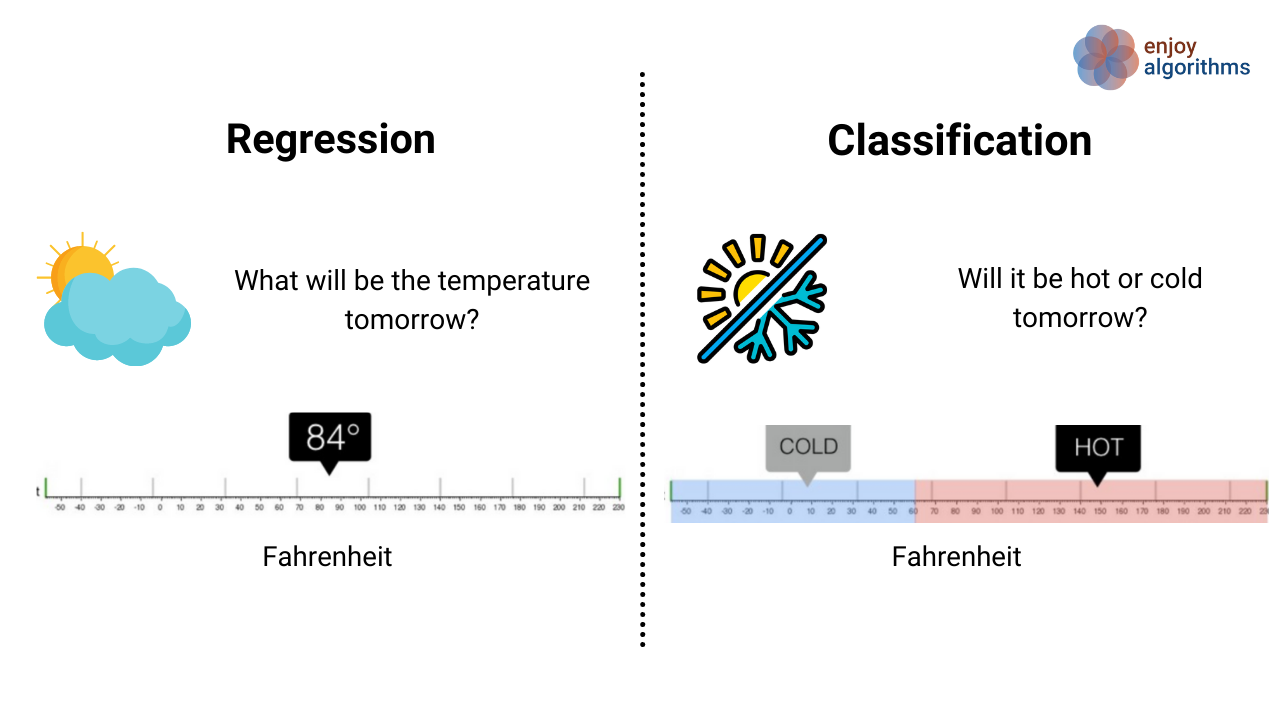
Let’s dive deeper into these two problems, one after the other.

Regression Problems in Machine Learning

Formal definition: Regression is a type of problem that uses machine learning algorithms to learn the continuous mapping function.

Taking the example shown in the above image, we want our machine learning algorithm to predict the weather temperature for today. The output would be continuous if we solved the above problem as a regression problem. It means our ML model will give exact temperature values, e.g., 24 °C, 24.5°C, 23°C etc.

Evaluation of Regression Models

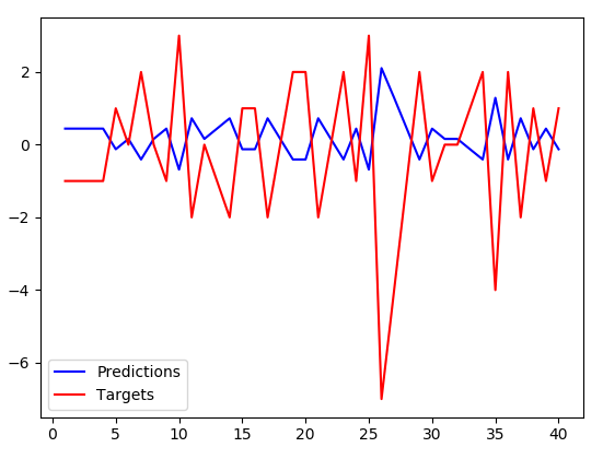
We measure the learned mapping function's performance by estimating the prediction’s closeness with the accurately labelled validation/test dataset. In the figure below, the regression model’s predicted values are blue, and red is the labelled function. The blue line’s closeness with the red line will give us a measure of How good is our model?

Cost Functions for Regression Problem

We need to define the cost function while building the regression model. It measures the value of the learned values’ deviation from the predicted values. Optimizers ensure this error reduces over the progressive iterations, also called epochs. Some of the most common error functions (or cost functions ) used for regression problems are:

• Mean Squared Error (MSE)

• Root Mean Squared Deviation/Error (RMSD/RMSE)

• Mean Absolute Error (MAE)

Note: Yi is the predicted value, Yi’ is the actual value, and N is the total samples over which the prediction is made.

Some Famous Examples of Regression Problems

• Predicting house prices based on the size of the house, availability of schools in the area, and other essential factors.
• Predicting a company's sales revenue based on previous sales data.
• Predicting the temperature of any day based on wind speed, humidity, and atmospheric pressure.

Popular Algorithms Used for Regression Problems

• Linear Regression
• Support Vector Regression
• Regression Tree: Decision Trees, Random Forests, etc.

Classification Problems in Machine Learning

In classification problems, the mapping function that algorithms want to learn is discrete. The objective is to find the decision boundary/boundaries, dividing the dataset into different categories. Classification is a type of problem that requires machine learning algorithms to learn how to assign a class label to the input data.

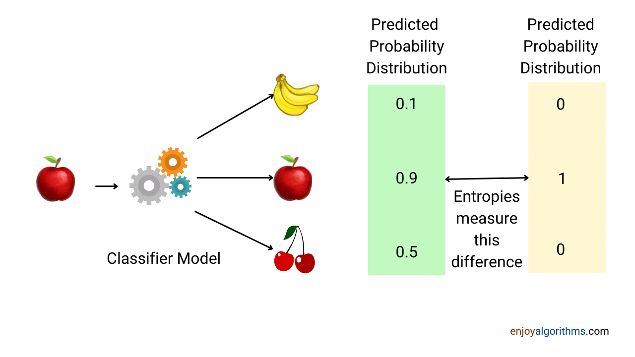
For example, suppose there are three class labels, [Apple, Banana, Cherry]. But the problem is that machines don’t have the sense to understand these labels. That’s why we need to convert these labels into a machine-readable format. For the above example, we can define Apple = [1,0,0], Banana = [0,1,0], and Cherry = [0,0,1]. Once the machine learns from these labelled training datasets, it will give probabilities of different classes on the test dataset like this: [P(Apple), P(Banana), P(Cherry)].

These predicted probabilities can be from one type of probability distribution function (PDF), and the actual (true) labelled dataset can be from another probability distribution function (PDF). If the predicted distribution function follows the exact distribution function, the model is learning accurately. Note: These PDF functions are continuous. As a similarity between classification and regression, if the predicted PDF follows the actual PDF, we can say the model learns the trends.

Some of the standard cost functions for the classification problems

• Categorical Cross-Entropy

Suppose there are M class labels, and the predicted distribution for the ith data sample is :

P(Y) = [Yi1', Yi2', ………. , YiM’]

And actual distribution for that sample would be:

A(Y) = [Yi1, Yi2, ……….., YiM]

Cross Entropy (CEi) =  — (Yi1*log(Yi1') + Yi2*log(Yi2') + …… + YiM*log(YiM’))

• Binary Cross-Entropy

This is a particular case of categorical cross-entropy, where there is only one output that can have two values, either 0 or 1. For example, if we want to predict whether a cat is present in any image or not.

Here, the cross-entropy function varies with the true value of Y,

CEi = -Yi1*log(Yi1') , if Yi1 = 1

CEi = -(1-Yi1)*log(1-Yi1'), if Yi1 = 0

And similarly, Binary-Cross-Entropy would be averaged over all the datasets.

The primary question we should ask ourselves is: If PDFs (probability distribution functions) are continuous in the range of [0,1], why can't MAE/MSE be chosen here? Take a pause and think!

Reason: MAE and MSE do well when the probability of an event occurring is close to the predicted value or when the wrong prediction's confidence is not that high. To understand the term confidence of prediction, let's take one example:

Suppose our ML model wrongly predicted that the patient does not have cancer, and our model predicted it with a probability of 0.9. We can say that our model is very much confident that the patient is cancer free, but he had cancer. Let's consider another scenario when the ML model says that a patient has cancer with a probability of 0.8, but this prediction is wrong. It is a case where the model predicts something wrong and is confident about the prediction. Our model must be penalized more for these predictions to address these cases. Right? Cost function values can ensure which prediction will be penalized more.

Let's calculate the cross-entropy (CE), MAE, and MSE of the case where the ML model is wrongly predicting that a patient has cancer with high confidence (Probability (Y')= 0.8). The actual output Y will be 0 here.

CE = -(1-Y)*log(1-Y’) = -(1–0)*log(1–0.8) = 1.64

MAE = |(Y-Y’)| = |0–0.8| = 0.8

MSE = |(Y-Y’)²| = (0–0.8)² = 0.64

As you can see, MAE and MSE have lower values than CE, meaning the Cost/Error function produces more value. Hence the model should be penalized more.

That’s why we needed different cost functions for the classification problems.

Most common evaluation metric for classification models

• Accuracy
• Confusion Matrix
• F1-Score
• Precision
• Recall etc. (We can find definitions here ). We will learn about these terms in greater detail in our later blogs.

Examples of classification problems

• Classifying if an email is spam or not, based on its content and how others have classified similar types of emails.
• Classifying a dog breed based on physical features such as height, width, and skin colour.
• Classifying whether today’s weather is hot or cold.

Algorithms for Classification

• Logistic Regression
• Support Vector Classification
• Decision Tree

Can we solve the same problem using regression as well as classification techniques?

Yes! We can. Let’s take one example.

Problem statement: Predict the steering angle of an autonomous vehicle based on the image data.

Constraints: The steering angle can take any value between -5⁰⁰ and 5⁰⁰ with a precision of ±⁵⁰.

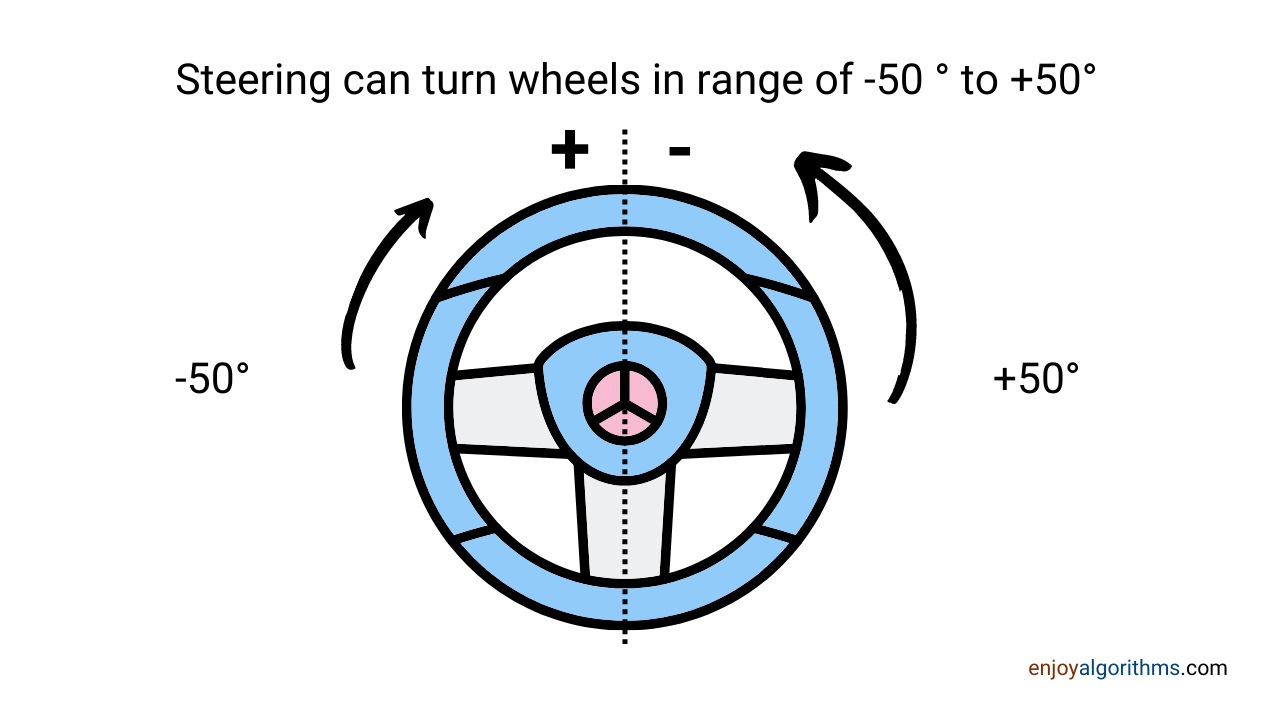
Regression Solution: This solution is simple, where we can map the images to the steering angle's continuous function, which continuously gives the output. Like steering angle = 20.7⁰ or steering angle = 5.0⁰.

Classification Problem: We stated that Precision is ±5⁰, so we can divide the range of -50⁰ to 50⁰ into 20 different classes by grouping every 5⁰ at a time.

Class 1 = -50⁰ to -46⁰

Class 2 = -45⁰ to 41⁰

…

Class 20 = 46⁰ to 50⁰

Now we have to classify the input image into these 20 classes. This way, the problem is converted into a classification problem. The performance reduces with the increment in the number of classes.

Critical Questions to Explore

1. What is the difference between classification and regression problems?
2. Why do we have different cost functions for different problem statements?
3. How do these cost functions decide whether the problem is a classification problem or a regression problem?
4. When do we use binary cross-entropy, and when do we use categorical cross-entropy?
5. Can you find more such problem statements that can be solved both ways?

Conclusion

In this article, we discussed classification and regression problems in detail. During this discussion, we explored the difference in cost functions like MAE, MSE, and Categorical Cross Entropies. Meanwhile, in the end, we analyzed a common problem statement that can be solved by considering the problem statement as a classification and a regression problem statement. We hope you have enjoyed the article and learned something new.

Enjoy Thinking, Enjoy Algorithms!